14.4 Differentiability and Tangent Planes
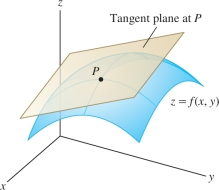
In this section, we generalize two basic concepts from single-variable calculus: differentiability and the tangent line. The tangent line becomes the tangent plane for functions of two variables (Figure 14.33).
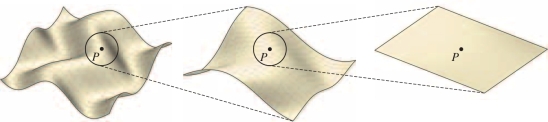
Intuitively, we would like to say that a continuous function \(f(x,y)\) is differentiable if it is locally linear—that is, if its graph looks flatter and flatter as we zoom in on a point \(P = (a,b,f(a,b))\) and eventually becomes indistinguishable from the tangent plane (Figure 14.34).
We can show that if the tangent plane at \(P=(a,b, f(a,b))\) exists, then its equation must be \(z=L(x,y)\), where \(L(x,y)\) is the linearization at \((a,b)\), defined by \[ \boxed{L(x,y)= f(a,b)+f_x(a,b)(x-a)+f_y(a,b)(y-b)} \]
Why must this be the tangent plane? Because it is the unique plane containing the tangent lines to the two vertical trace curves through \(P\) [Figure 14.35]. Indeed, when we set \(y=b\) in \(z = L(x,y)\), the term \(f_y(a,b)(y-b)\) drops out and we are left with the equation of the tangent line to the vertical trace \(z = f(x,b)\) at \(P\): \[ z=L(x,b) = f(a,b) +f_x(a,b)(x-a) \]
Similarly, \(z=L(a,y)\) is the tangent line to the vertical trace \(z = f(a,y)\) at \(P\).
806
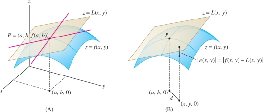
Before we can say that the tangent plane exists, however, we must impose a condition on \(f(x,y)\) guaranteeing that the graph looks flat as we zoom in on \(P\). Set \[ e(x,y) = f(x,y) - L(x,y) \]
As we see in Figure 14.35, \(|e(x,y)|\) is the vertical distance between the graph of \(f(x,y)\) and the plane \(z=L(x,y)\). This distance tends to zero as \((x,y)\) approaches \((a,b)\) because \(f(x,y)\) is continuous. To be locally linear, we require that the distance tend to zero faster than the distance from \((x,y)\) to \((a,b)\). We express this by the requirement \[ \lim_{(x,y)\to(a,b)}\frac{e(x,y)}{\sqrt{(x-a)^2+(y-b)^2}}=0 \]
DEFINITION Differentiability
Assume that \(f(x,y)\) is defined in a disk \(D\) containing \((a,b)\) and that \(f_x(a,b)\) and \(f_y(a,b)\) exist.
- \(f(x,y)\) is differentiable at \((a,b)\) if it is locally linear—that is, if \begin{equation*} f(x,y) = L(x,y) + e(x,y)\tag{1} \end{equation*} where \(e(x,y)\) satisfies \[ {\lim_{(x,y)\to(a,b)}\frac{e(x,y)}{\sqrt{(x-a)^2+(y-b)^2}}=0} \]
- In this case, the tangent plane to the graph at \((a,b,f(a,b))\) is the plane with equation \(z=L(x,y)\). Explicitly, \begin{equation*} \boxed{z = f(a,b)+f_x(a,b)(x-a)+f_y(a,b)(y-b)}\tag{2} \end{equation*}
REMINDER
\[ \begin{array}{l} L(x,y) = f(a,b) + f_x(a,b)(x-a)\\ \qquad\qquad\qquad +f_y(a,b)(y-b) \end{array} \]
If \(f(x,y)\) is differentiable at all points in a domain \({\mathcal{D}}\), we say that \(f(x,y)\) is differentiable on \({\mathcal{D}}\).
It is cumbersome to check the local linearity condition directly (see Exercise 41), but fortunately, this is rarely necessary. The following theorem provides a criterion for differentiability that is easy to apply. It assures us that most functions arising in practice are differentiable on their domains. See Appendix D for a proof.
The definition of differentiability extends to functions of \(n\)-variables, and Theorem 1 holds in this setting: If all of the partial derivatives of \(f(x_1,\ldots,x_n)\) exist and are continuous on an open domain \({\mathcal{D}}\), then \(f(x_1,\ldots,x_n)\) is differentiable on \({\mathcal{D}}\).
THEOREM 1 Criterion for Differentiability
If \(f_x(x,y)\) and \(f_y(x,y)\) exist and are continuous on an open disk \(D\), then \(f(x,y)\) is differentiable on \(D\).
807
EXAMPLE 1
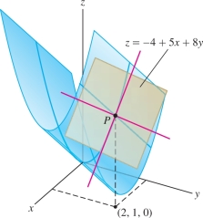
Show that \(f(x,y) = 5x+4y^2\) is differentiable (Figure 14.36). Find the equation of the tangent plane at \((a,b) = (2,1)\).
Solution The partial derivatives exist and are continuous functions: \[ f(x,y) = 5x+4y^2, \qquad f_x(x,y) = 5, \qquad f_y(x,y) = 8y \]
Therefore, \(f(x,y)\) is differentiable for all \((x,y)\) by Theorem 1. To find the tangent plane, we evaluate the partial derivatives at \((2,1)\): \[ f(2,1) = 14, \qquad f_x(2,1) = 5, \qquad f_y(2,1) = 8 \]
The linearization at \((2,1)\) is \[ L(x,y) = \underbrace{14+5(x-2)+8(y-1)}_{f(a,b)+f_x(a,b)(x-a) + f_y(a,b)(y-b)} = -4+5x+8y \]
The tangent plane through \(P=(2,1,14)\) has equation \(z = -4+5x+8y\).
Assumptions Matter Local linearity plays a key role, and although most reasonable functions are locally linear, the mere existence of the partial derivatives does not guarantee local linearity. This is in contrast to the one-variable case, where \(f(x)\) is automatically locally linear at \(x=a\) if \(f'(a)\) exists (Exercise 44).
Local linearity is used in the next section to prove the Chain Rule for Paths, upon which the fundamental properties of the gradient are based.
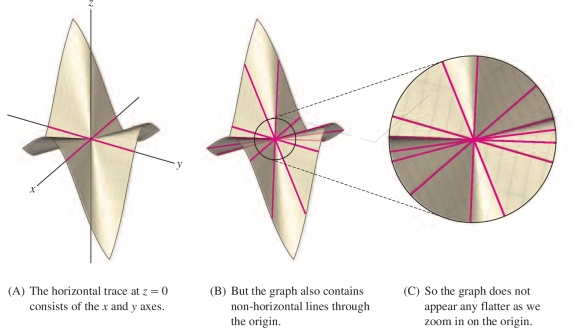
The function \(g(x,y)\) in Figure 14.37 shows what can go wrong. The graph contains the \(x\)- and \(y\)-axes—in other words, \(g(x,y) =0\) if \(x\) or \(y\) is zero—and therefore, the partial derivatives \(g_x(0,0)\) and \(g_y(0,0)\) are both zero. The tangent plane at the origin \((0,0)\), if it existed, would have to be the \(xy\)-plane. However, Figure 14.37 shows that the graph also contains lines through the origin that do not lie in the \(xy\)-plane (in fact, the graph is composed entirely of lines through the origin). As we zoom in on the origin, these lines remain at an angle to the \(xy\)-plane, and the surface does not get any flatter. Thus \(g(x,y)\) cannot be locally linear at \((0,0)\), and the tangent plane does not exist. In particular, \(g(x,y)\) cannot satisfy the assumptions of Theorem 1, so the partial derivatives \(g_x(x,y)\) and \(g_y(x,y)\) cannot be continuous at the origin (see Exercise 45 for details).
808
EXAMPLE 2
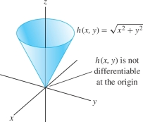
Where is \(h(x,y) =\sqrt{x^2+y^2}\) differentiable?
Solution The partial derivatives exist and are continuous for all \((x,y)\ne (0,0)\): \[ h_x(x,y) = \frac{x}{\sqrt{x^2+y^2}} ,\qquad h_y(x,y) = \frac{y}{\sqrt{x^2+y^2}} \]
However, the partial derivatives do not exist at \((0,0)\). Indeed, \(h_x(0,0)\) does not exist because \(h(x,0) = \sqrt{x^2}=|x|\) is not differentiable at \(x=0\). Similarly, \(h_y(0,0)\) does not exist. By Theorem 1, \(h(x,y)\) is differentiable except at \((0,0)\) (Figure 14.38).
EXAMPLE 3
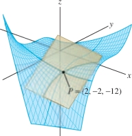
Find a tangent plane of the graph of \(f(x,y)= xy^3 + x^2\) at \((2,-2)\).
Solution The partial derivatives are continuous, so \(f(x,y)\) is differentiable: \[ \begin{array}{llll} f_x(x,y)&= y^3+2x,&\qquad f_x(2,-2)&= -4 \\ f_y(x,y) &= 3xy^2, &\qquad f_y(2,-2) &=24 \end{array} \]
Since \(f(2,-2)=-12\), the tangent plane through \((2,-2,-12)\) has equation \[ \begin{array}{rl} z &= -12 - 4 (x-2) + 24 (y+2) \end{array} \]
This can be rewritten as \(z = 44 - 4 x + 24 y\) (Figure 14.39).
Linear Approximation and Differentials
By definition, if \(f(x,y)\) is differentiable at \((a,b)\), then it is locally linear and the linear approximation is \[ \boxed{f(x,y)\approx L(x,y) \qquad \textrm{for }(x,y)\textrm{ near }(a,b)} \] where \[ L(x,y) = f(a,b)+f_x(a,b)(x-a) + f_y(a,b)(y-b) \]
We shall rewrite this in several useful ways. First, set \(x=a+h\) and \(y=b+k\). Then \begin{equation*} \boxed{ f(a+h,b+k) \approx f(a,b)+f_x(a,b)h + f_y(a,b)k}\tag{3} \end{equation*}
We can also write the linear approximation in terms of the change in \(f\): \[ \displaystyle \Delta f = f(x,y)-f(a,b),\qquad \Delta x = x-a,\qquad \Delta y = y-b \] \begin{equation*} \displaystyle \boxed{\Delta f \approx f_x(a,b)\Delta x + f_y(a,b)\Delta y}\tag{4} \end{equation*}
Finally, the linear approximation is often expressed in terms of differentials: \[ \boxed{ df = f_x(x,y)\,dx +f_y(x,y)\,dy = \frac{\partial f}{\partial x} dx + \frac{\partial f}{\partial y} dy } \]
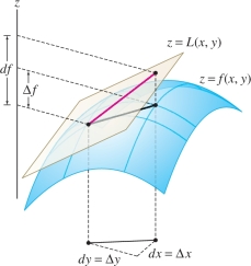
As shown in Figure 14.40, \(df\) represents the change in height of the tangent plane for given changes \(dx\) and \(dy\) in \(x\) and \(y\) (when we work with differentials, we call them \(dx\) and \(dy\) instead of \(\Delta x\) and \(\Delta y\)), whereas \(\Delta f\) is the change in the function itself. The linear approximation tells us that the two changes are approximately equal: \[ \Delta f \approx df \]
809
These approximations apply in any number of variables. In three variables, \[ f(a+h,b+k,c+\ell)\approx f(a,b,c)+f_x(a,b,c)h+f_y(a,b,c)k+f_z(a,b,c)\ell \] or in terms of differentials, \(\Delta f\approx df\), where \[ df = f_x(x,y,z)\,dx +f_y(x,y,z)\,dy +f_z(x,y,z)\,dz \]
REMINDER
The percentage error is equal to \[ \left|\frac{\textrm{error}}{\textrm{actual value}}\right|\times 100\% \]
EXAMPLE 4
Use the linear approximation to estimate \[ (3.99)^3(1.01)^4(1.98)^{-1} \]
Then use a calculator to find the percentage error.
Solution Think of \((3.99)^3(1.01)^4(1.98)^{-1}\) as a value of \(f(x,y,z) = x^3y^4z^{-1}\): \[ f(3.99,1.01,1.98) = (3.99)^3(1.01)^4(1.98)^{-1} \]
Then it makes sense to use the linear approximation at \((4,1,2)\): \[ \begin{array}{llll} f(x,y,z) &= x^3y^4z^{-1},&\qquad &f(4,1,2) = (4^3)(1^4)(2^{-1})=32 \\ f_x(x,y,z) &= 3x^2y^4z^{-1},& \qquad & f_x(4,1,2) = 24 \\ f_y(x,y,z) &= 4x^3y^3z^{-1},& \qquad & f_y(4,1,2) =128\\ f_z(x,y,z) &= -x^3y^4z^{-2},& \qquad & f_z(4,1,2) = -16 \end{array} \]
The linear approximation in three variables stated above, with \(a=4\), \(b=1\), \(c=2\), gives us \[ \underbrace{(4+h)^3(1+k)^4(2+\ell)^{-1}}_{f(4+h,1+k,2+\ell)} \approx 32 + 24h+128k-16\ell \]
For \(h=-0.01\), \(k=0.01\), and \(\ell = -0.02\), we obtain the desired estimate \[ (3.99)^3(1.01)^4(1.98)^{-1} \approx 32+24(-0.01)+128(0.01)-16(-0.02) = 33.36 \]
The calculator value is \((3.99)^3(1.01)^4(1.98)^{-1}\approx 33.384\), so the error in our estimate is less than 0.025. The percentage error is \[ \textrm{Percentage error} \approx \frac{|33.384 - 33.36|}{33.384}\times 100 \approx 0.075 \% \]
EXAMPLE 5 Body Mass Index
A person’s BMI is \(I = W/H^2\), where \(W\) is the body weight (in kilograms) and \(H\) is the body height (in meters). Estimate the change in a child’s BMI if \((W,H)\) changes from \((40, 1.45)\) to \((41.5,1.47)\).
BMI is one factor used to assess the risk of certain diseases such as diabetes and high blood pressure. The range \(18.5 \le I\le 24.9\) is considered normal for adults over 20 years of age.
Solution
Step 1. Compute the differential at \((W,H)=(40,1.45)\) \[ \begin{array}{llll} &\frac{\partial I}{\partial W} = \frac{\partial }{\partial W}\left(\frac{W}{H^2}\right) = \frac{1}{H^2}, &\qquad &\frac{\partial I}{\partial H} = \frac{\partial }{\partial H}\left(\frac{W}{H^2}\right) = -\frac{2W}{H^3} \end{array} \] At \((W,H) = (40,1.45)\), we have \[ \begin{array}{llll} &\frac{\partial I}{\partial W}\bigg|_{(40,1.45)}=\frac1{1.45^2} \approx 0.48, &\qquad & \frac{\partial I}{\partial H}\bigg|_{(40,1.45)}=-\frac{2(40)}{1.45^3}\approx -26.24 \end{array} \]
Therefore, the differential at \((40,1.45)\) is \[ dI \approx 0.48\,dW -26.24\,d\!H \]
810
Step 2. Estimate the change
We have shown that the differential \(dI\) at \((40,1.45)\) is \(0.48\, dW - 26.24\, d\!H\). If \((W,H)\) changes from \((40,1.45)\) to \((41.5,1.47)\), then \[ dW = 41.5-40 = 1.5,\qquad dH = 1.47 - 1.45= 0.02 \]
Therefore, \[ \Delta I \approx dI = 0.48\,dW -26.24\,d\!H = 0.48 (1.5) - 26.24 (0.02)\approx 0.2 \]
We find that BMI increases by approximately \(0.2\).
14.4.1 Summary
- The linearization in two and three variables: \[ \begin{array}{rl} L(x,y)&=f(a,b)+f_x(a,b)(x-a)+f_y(a,b)(y-b)\\ L(x,y,z) &= f(a,b,c)+f_x(a,b,c)(x-a)+f_y(a,b,c)(y-b)+f_z(a,b,c)(z-c) \end{array} \]
- \(f(x,y)\) is differentiable at \((a,b)\) if \(f_x(a,b)\) and \(f_y(a,b)\) exist and \[ f(x,y)=L(x,y)+ e(x,y) \] where \(e(x,y)\) is a function such that \[ {\lim_{(x,y)\to(a,b)}\frac{e(x,y)}{\sqrt{(x-a)^2+(y-b)^2}}=0} \]
- Result used in practice: If \(f_x(x,y)\) and \(f_y(x,y)\) exist and are continuous in a disk \(D\) containing \((a,b)\), then \(f(x,y)\) is differentiable at \((a,b)\).
- Equation of the tangent plane to \(z=f(x,y)\) at \((a,b)\): \[ z = f(a,b) + f_x(a,b)(x-a)+f_y(a,b)(y-b) \]
- Equivalent forms of the linear approximation: \[ \begin{array}{rl} f(x,y) &\approx f(a,b)+f_x(a,b)(x-a)+f_y(a,b)(y-b)\\ f(a+h,b+k) &\approx f(a,b)+f_x(a,b)h+f_y(a,b)k\\ \Delta f &\approx f_x(a,b)\,\Delta x+f_y(a,b)\,\Delta y \end{array} \]
- In differential form, \(\Delta f\approx df\), where \[ \begin{array}{rl} df &= f_x(x,y)\,dx +f_y(x,y)\,dy = \frac{\partial f}{\partial x} dx + \frac{\partial f}{\partial y} dy \\ df &= f_x(x,y,z)\,dx +f_y(x,y,z)\,dy +f_z(x,y,z)\,dz = \frac{\partial f}{\partial x} dx + \frac{\partial f}{\partial y} dy + \frac{\partial f}{\partial z} dz \end{array} \]