14.5 The Gradient and Directional Derivatives
We have seen that the rate of change of a function \(f\) of several variables depends on a choice of direction. Since directions are indicated by vectors, it is natural to use vectors to describe the derivative of \(f\) in a specified direction.
To do this, we introduce the gradient \(\nabla f_P\), which is the vector whose components are the partial derivatives of \(f\) at \(P\).
The gradient of a function of \(n\) variables is the vector \[ \nabla f = \left\langle\frac{\partial f}{\partial x_1},\frac{\partial f}{\partial x_2},\ldots,\frac{\partial f}{\partial x_n}\right\rangle \]
DEFINITION The Gradient
The gradient of a function \(f(x,y)\) at a point \(P=(a,b)\) is the vector \[ \boxed{\nabla f_P = \left\langle f_x(a,b), f_y(a,b)\right\rangle} \]
In three variables, if \(P=(a,b,c)\), \[ \boxed{\nabla f_P = \left\langle f_x(a,b,c), f_y(a,b,c), f_z(a,b,c)\right\rangle} \]
We also write \(\nabla f_{(a,b)}\) or \(\nabla f(a,b)\) for the gradient. Sometimes, we omit reference to the point \(P\) and write \[ \nabla f = \left\langle \frac{\partial f}{\partial x},\frac{\partial f}{\partial y} \right\rangle \qquad\textrm{or}\qquad \nabla f = \left\langle \frac{\partial f}{\partial x},\frac{\partial f}{\partial y},\frac{\partial f}{\partial z} \right\rangle \]
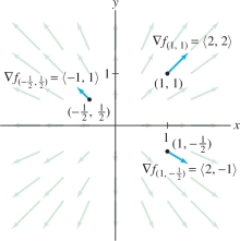
The gradient \(\nabla f\) “assigns” a vector \(\nabla f_P\) to each point in the domain of \(f\), as in Figure 14.41.
The symbol \(\nabla\), called “del,” is an upside-down Greek delta. It was popularized by the Scottish physicist P. G. Tait (1831–1901), who called the symbol “nabla,” because of its resemblance to an ancient Assyrian harp. The great physicist James Clerk Maxwell was reluctant to adopt this term and would refer to the gradient simply as the “slope.” He wrote jokingly to his friend Tait in 1871, “Still harping on that nabla?”
EXAMPLE 1 Drawing Gradient Vectors
Let \(f(x,y)=x^2+y^2\). Calculate the gradient \(\nabla f\), draw several gradient vectors, and compute \(\nabla f_P\) at \(P=(1,1)\).
Solution The partial derivatives are \(f_x(x,y)=2x\) and \(f_y(x,y)=2y\), so \[ \nabla f = \left\langle 2x,2y\right\rangle \]
The gradient attaches the vector \(\left\langle 2x,2y\right\rangle\) to the point \((x,y)\). As we see in Figure 14.41, these vectors point away from the origin. At the particular point \((1,1)\), \[ \nabla f_P = \nabla f(1,1) = \left\langle 2, 2\right\rangle \]
EXAMPLE 2 Gradient in Three Variables
Calculate \(\nabla f_{(3,-2,4)}\), where \[ f(x,y,z)=ze^{2x+3y} \]
Solution The partial derivatives and the gradient are \[ \begin{array}{rl} \frac{\partial f}{\partial x} &=2ze^{2x+3y},\qquad \frac{\partial f}{\partial y} = 3ze^{2x+3y},\qquad \frac{\partial f}{\partial z} = e^{2x+3y}\\ \nabla f &= \big\langle 2ze^{2x+3y}, 3ze^{2x+3y}, e^{2x+3y}\big\rangle \end{array} \]
Therefore, \(\nabla f_{(3,-2,4)} = \big\langle 2\cdot 4e^{0}, 3\cdot 4e^{0}, e^{0} \big\rangle = \left\langle 8, 12, 1\right\rangle\).
The following theorem lists some useful properties of the gradient. The proofs are left as exercises (see Exercises 62–64).
814
THEOREM 1 Properties of the Gradient
If \(f(x,y,z)\) and \(g(x,y,z)\) are differentiable and \(c\) is a constant, then
- (i) \(\nabla(f+g)= \nabla f + \nabla g\)
- (ii) \(\nabla(cf)= c\nabla f \)
- (iii) Product Rule for Gradients: \(\nabla(fg)= f\nabla g + g\nabla f \)
- (iv)Chain Rule for Gradients: If \(F(t)\) is a differentiable function of one variable, then \begin{equation*} \nabla(F(f(x,y,z)))= F'(f(x,y,z))\nabla f\tag{1} \end{equation*}
EXAMPLE 3 Using the Chain Rule for Gradients
Find the gradient of \[ g(x,y,z)=(x^2+y^2+z^2)^8 \]
Solution The function \(g\) is a composite \(g(x,y,z)=F(f(x,y,z))\) with \(F(t)=t^8\) and \(f(x,y,z)=x^2+y^2+z^2\) and apply Eq. (1): \[ \begin{array}{rl} \nabla g = \nabla \big((x^2+y^2+z^2)^8 \big) &= 8(x^2+y^2+z^2)^7\nabla(x^2+y^2+z^2) \\ &=8(x^2+y^2+z^2)^7\left\langle 2x, 2y, 2z\right\rangle\\& = 16(x^2+y^2+z^2)^7\left\langle x, y, z\right\rangle \end{array} \]
The Chain Rule for Paths
Our first application of the gradient is the Chain Rule for Paths. In Chapter 13, we represented a path in \({\bf{R}}^3\) by a vector-valued function \({\bf{r}}(t) = \left\langle x(t), y(t), z(t)\right\rangle\). It is convenient to use a slightly different notation in this chapter.
A path will be represented by a function \({\bf{c}}(t) = (x(t),y(t),z(t))\). We think of \({\bf{c}}(t)\) as a moving point rather than as a moving vector (Figure 14.42). By definition, \({\bf{c}}'(t)\) is the vector of derivatives as before: \[ \boxed{{\bf{c}}(t) = (x(t),y(t),z(t)),\qquad {\bf{c}}'(t) = \big\langle x'(t),y'(t),z'(t)\big\rangle} \]
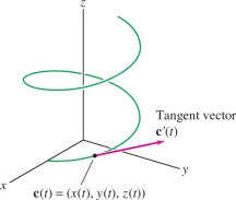
Recall from Section 13.2 that \({\bf{c}}'(t)\) is the tangent or “velocity” vector that is tangent to the path and points in the direction of motion. We use similar notation for paths in \({\bf{R}}^2\).
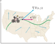
The Chain Rule for Paths deals with composite functions of the type \(f({\bf{c}}(t))\). What is the idea behind a composite function of this type? As an example, suppose that \(T(x,y)\) is the temperature at location \((x,y)\) (Figure 14.43). Now imagine a biker—we'll call her Chloe—riding along a path \({\bf{c}}(t)\). We suppose that Chloe carries a thermometer with her and checks it as she rides. Her location at time \(t\) is \({\bf{c}} (t)\), so her temperature reading at time \(t\) is the composite function \[ T({\bf{c}}(t)) = \textrm{Chloe’s temperature at time }t \]
The temperature reading varies as Chloe’s location changes, and the rate at which it changes is the derivative \[ \frac{d }{d t}T({\bf{c}}(t)) \]
The Chain Rule for Paths tells us that this derivative is simply the dot product of the temperature gradient \(\nabla T\) evaluated at \({\bf{c}}(t)\) and Chloe’s velocity vector \({\bf{c}}'(t)\).
815
THEOREM 2 Chain Rule for Paths
If \(f\) and \({\bf{c}}(t)\) are differentiable, then \[ \boxed{ \frac{d }{d t}f({\bf{c}}(t)) = \nabla f_{{\bf{c}}(t)}{\cdot} {\bf{c}}'(t)} \]
Explicitly, in the case of two variables, if \({\bf{c}}(t) = (x(t),y(t))\), then \[ \frac{d }{d t}f({\bf{c}}(t)) = \left\langle \frac{\partial f}{\partial x},\frac{\partial f}{\partial y} \right\rangle{\cdot} \left\langle x'(t),y'(t) \right\rangle= \frac{\partial f}{\partial x}\frac{d x}{d t} + \frac{\partial f}{\partial y} \frac{d y}{d t} \]
CAUTION
Do not confuse the Chain Rule for Paths with the more elementary Chain Rule for Gradients stated in Theorem 1 above.
Proof By definition, \[ \frac{d }{d t}f({\bf{c}}(t)) = \lim_{h\to 0}\frac{f(x(t+h),y(t+h))-f(x(t),y(t))}h \] To calculate this derivative, set \[ \Delta f =f(x(t+h),y(t+h))-f(x(t),y(t))\\ \Delta x = x(t+h)-x(t),\quad\quad \Delta y = y(t+h)-y(t) \]
The proof is based on the local linearity of \(f\). As in Section 14.4, we write \[ \Delta f = f_x(x(t),y(t)) \Delta x + f_y(x(t),y(t))\Delta y + e(x(t+h),y(t+h)) \]
Now set \(h=\Delta t\) and divide by \(\Delta t\): \[ \frac{\Delta f}{\Delta t} =f_x(x(t),y(t))\frac{\Delta x}{\Delta t} + f_y(x(t),y(t))\frac{\Delta y}{\Delta t} + \frac{e(x(t+\Delta t),y(t+\Delta t))}{\Delta t} \]
Suppose for a moment that the last term tends to zero as \(\Delta t\to 0\). Then we obtain the desired result: \[ \begin{array}{rl} \frac{d }{d t}f({\bf{c}}(t)) & = \lim_{\Delta t\to 0}\frac{\Delta f}{\Delta t}\\ &=f_x(x(t),y(t))\lim_{\Delta t\to 0}\frac{\Delta x}{\Delta t}+f_y(x(t),y(t))\lim_{\Delta t\to 0}\frac{\Delta y}{\Delta t}\\ &=f_x(x(t),y(t))\frac{d x}{d t} + f_y(x(t),y(t))\frac{d y}{d t} \\&= \nabla f_{{\bf{c}}(t)}{\cdot} {\bf{c}}'(t) \end{array} \]
We verify that the last term tends to zero as follows: \[ \begin{array}{rl} \lim_{\Delta t\to 0}&\frac{e(x(t+\Delta t),y(t+\Delta t))}{\Delta t} =\lim_{\Delta t\to 0}\frac{e(x(t+\Delta t),y(t+\Delta t))}{\sqrt{(\Delta x)^2+(\Delta y)^2}} \left(\frac{\sqrt{(\Delta x)^2+(\Delta y)^2}}{\Delta t}\right)\\ &=\underbrace{\left(\lim_{\Delta t\to 0}\frac{e(x(t+\Delta t),y(t+\Delta t))}{\sqrt{(\Delta x)^2+(\Delta y)^2}}\right)}_{\textrm{Zero}} \lim_{\Delta t\to 0}\left(\sqrt{\left(\frac{\Delta x}{\Delta t}\right)^2+\left(\frac{\Delta y}{\Delta t}\right)^2} \right)=0 \end{array} \]
The first limit is zero because a differentiable function is locally linear (Section 14.4). The second limit is equal to \(\sqrt{x'(t)^2+y'(t)^2}\), so the product is zero.
816
EXAMPLE 4
The temperature at location \((x,y)\) is \(T(x,y)=20+10e^{-0.3(x^2+y^2)}{}^\circ\mathrm{C}\). A bug carries a tiny thermometer along the path \[ {\bf{c}}(t) = (\cos(t-2), \sin 2t) \] (\(t\) in seconds) as in Figure 14.44. How fast is the temperature changing at \(t=0.6\) s?
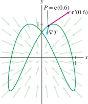
Solution At \(t=0.6\) s, the bug is at location \[ {\bf{c}}(0.6) = (\cos (-1.4), \sin 0.6)\approx (0.170,0.932)\\ \]
By the Chain Rule for Paths, the rate of change of temperature is the dot product \[ \frac{d T}{d t}\bigg|_{t=0.6} =\nabla T_{{\bf{c}}(0.6)}{\cdot} {\bf{c}}'(0.6) \]
We compute the vectors \[ \begin{array}{rl} \nabla T &= \left\langle -6xe^{-0.3(x^2+y^2)},-6ye^{-0.3(x^2+y^2)}\right\rangle\\ {\bf{c}}'(t) &= \left\langle -\sin(t-2),2\cos 2t\right\rangle \end{array} \] and evaluate at \({\bf{c}}(0.6) =(0.170,0.932)\) using a calculator: \[ \begin{array}{rl} \nabla T_{{\bf{c}}(0.6)} &\approx \left\langle -0.779, -4.272\right\rangle\\ {\bf{c}}'(0.6) &\approx \left\langle 0.985, 0.725 \right\rangle \end{array} \]
Therefore, the rate of change is \[ \begin{array}{rl} \frac{d T}{d t}\bigg|_{t=0.6} \nabla T_{{\bf{c}}(0.6)} \cdot {\bf{c}}'(t)& \approx \left\langle -0.779, -4.272 \right\rangle{\cdot} \left\langle 0.985, 0.725 \right\rangle \approx -3.87^{\circ}\text{C/s} \end{array} \]
In the next example, we apply the Chain Rule for Paths to a function of three variables. In general, if \(f(x_1,\dots,x_n)\) is a differentiable function of \(n\) variables and \({\bf{c}}(t)=(x_1(t),\dots,x_n(t))\) is a differentiable path, then \[ \frac{d }{d t}f({\bf{c}}(t)) = \nabla f{\cdot} {\bf{c}}'(t) = \frac{\partial f}{\partial x_1}\frac{d x_1}{d t}+ \frac{\partial f}{\partial x_2}\frac{d x_2}{d t}+ \cdots+ \frac{\partial f}{\partial x_n}\frac{d x_n}{d t} \]
EXAMPLE 5
Calculate \(\frac{d }{d t}f({\bf{c}}(t))\bigg|_{t =\pi/2}\), where \[ f(x,y,z)=xy+z^2\qquad\hbox{and}\qquad {\bf{c}}(t)=(\cos t,\sin t,t) \]
Solution We have \({\bf{c}}\big(\frac{\pi}2\big) = \big(\cos \frac{\pi}2,\sin \frac{\pi}2,\frac{\pi}2\big) = \big(0,1,\frac{\pi}2\big)\). Compute the gradient: \[ \nabla f = \left\langle \frac{\partial f}{\partial x}, \frac{\partial f}{\partial y},\frac{\partial f}{\partial z} \right\rangle = \left\langle y , x , 2z\right\rangle, \qquad \nabla f_{{\bf{c}}(\pi/2)} = \nabla f \left(0,1,\frac{\pi}2\right) = \left\langle 1,0,\pi\right\rangle \]
Then compute the tangent vector: \[ {\bf{c}}'(t) = \left\langle {-\sin t}, \cos t, 1\right\rangle,\qquad {\bf{c}}'\left(\frac{\pi}2\right) = \left\langle {-\sin \frac{\pi}2}, \cos \frac{\pi}2, 1\right\rangle = \left\langle -1,0,1\right\rangle \]
By the Chain Rule, \[ \frac{d }{d t} f({\bf{c}}(t))\bigg|_{t=\pi/2} = \nabla f_{{\bf{c}}(\pi/2)}{\cdot} {\bf{c}}'\left(\frac{\pi}2\right) = \left\langle 1,0,\pi\right\rangle{\cdot}\left\langle -1,0,1\right\rangle = \pi-1 \]
817
Directional Derivatives
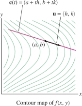
We come now to one of the most important applications of the Chain Rule for Paths. Consider a line through a point \(P=(a,b)\) in the direction of a unit vector \({\bf{u}}=\left\langle h, k\right\rangle\) (see Figure 14.45): \[ {\bf{c}}(t) = (a+th,b+tk) \]
The derivative of \(f({\bf{c}}(t))\) at \(t=0\) is called the directional derivative of f with respect to \({\bf{u}}\) at P, and is denoted \(D_{{\bf{u}}}f(P)\) or \(D_{{\bf{u}}}f(a,b)\): \[ D_{{\bf{u}}} f(a,b) = \frac{d }{d t}f({\bf{c}}(t))\bigg|_{t=0} = \lim_{t\to 0} \frac{f(a+th,b+tk) - f(a,b)}t \]
Directional derivatives of functions of three or more variables are defined in a similar way.
DEFINITION Directional Derivative
The directional derivative in the direction of a unit vector \({\bf{u}} = \left\langle h,k\right\rangle\) is the limit (assuming it exists) \[ \boxed{D_{{\bf{u}}} f(P) = D_{{\bf{u}}}f(a,b) = \lim_{t\to 0} \frac{f(a+th,b+tk) - f(a,b)}t} \]
Note that the partial derivatives are the directional derivatives with respect to the standard unit vectors \({\bf{i}} = \left\langle 1,0\right\rangle\) and \({\bf{j}}=\left\langle 0,1\right\rangle\). For example, \[ \begin{array}{rl} D_{{\bf{i}}}f(a,b) &= \lim_{t\to 0} \frac{f(a+t(1),b+t(0)) - f(a,b)}t = \lim_{t\to 0} \frac{f(a+t,b) - f(a,b)}t\\ & = f_x(a,b) \end{array} \]
Thus we have \[ f_x(a,b) = D_{{\bf{i}}}f(a,b),\qquad f_y(a,b) = D_{{\bf{j}}}f(a,b) \]
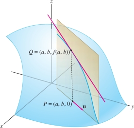
CONCEPTUAL INSIGHT
The directional derivative \(D_{{\bf{u}}}f(P)\) is the rate of change of \(f\) per unit change in the horizontal direction of \({\bf{u}}\) at \(P\) (Figure 14.46). This is the slope of the tangent line at \(Q\) to the trace curve obtained when we intersect the graph with the vertical plane through \(P\) in the direction \({\bf{u}}\).
818
To evaluate directional derivatives, it is convenient to define \(D_{{\bf{v}}}f(a,b)\) even when \({\bf{v}}=\left\langle h,k\right\rangle\) is not a unit vector: \[ D_{{\bf{v}}} f(a,b) = \frac{d }{d t}f({\bf{c}}(t))\bigg|_{t=0} = \lim_{t\to 0} \frac{f(a+th,b+tk) - f(a,b)}t \]
We call \(D_{{\bf{v}}}f\) the derivative with respect to \({\bf{v}}\).
If we set \({\bf{c}}(t) = (a+th,b+tk)\), then \(D_{{\bf{v}}}f(a,b)\) is the derivative at \(t = 0\) of the composite function \(f({\bf{c}}(t))\), where \({\bf{c}}(t) = (a+th,b+tk)\), and we can evaluate it using the Chain Rule for Paths. We have \({\bf{c}}'(t)=\left\langle h,k\right\rangle = {\bf{v}}\), so \[ D_{{\bf{v}}}f(a,b) = \nabla f_{(a,b)}{\cdot} {\bf{c}}'(0) =\nabla f_{(a,b)}{\cdot} {\bf{v}} \]
This yields the basic formula: \begin{equation*} \boxed{ D_{{\bf{v}}}f(a,b) = \nabla f_{(a,b)}{\cdot}{\bf{v}} }\tag{2} \end{equation*}
Similarly, in three variables, \( D_{{\bf{v}}} f(a,b,c) = \nabla f_{(a,b,c)}{\cdot} {\bf{v}}\).
For any scalar \(\lambda\), \(D_{\lambda {\bf{v}}}f(P)=\nabla f_P{\cdot}(\lambda {\bf{v}}) = \lambda \nabla f_P{\cdot} {\bf{v}} \). Therefore, \begin{equation*} \boxed{D_{\lambda {\bf{v}}}f(P) = \lambda D_{{\bf{v}}}f(P)}\tag{3} \end{equation*}
If \({\bf{v}} \neq \mathbf{0}\), then \({\bf{u}}= \frac1{\left \| {\bf{v}} \right \|}{\bf{v}}\) is a unit vector in the direction of \({\bf{v}}\). Applying Eq. (3) with \(\lambda= {1}/{\|{\bf{u}}\|}\) gives us a formula for the directional derivative \(D_{{\bf{u}}}f(P)\) in terms of \(D_{{\bf{v}}}f(P)\).
THEOREM 3 Computing the Directional Derivative
If \({\bf{v}}\ne \mathbf{0}\), then \({\bf{u}}={{\bf{v}}}/{\left \| {\bf{v}} \right \|}\) is the unit vector in the direction of \({\bf{v}}\), and the directional derivative is given by \begin{equation*} \boxed{D_{{\bf{u}}}f(P) = \frac{1}{\left \| {\bf{v}} \right \|}\nabla f_{P}{\cdot} {\bf{v}}}\tag{4} \end{equation*}
EXAMPLE 6
Let \(f(x,y) = xe^{y}\), \(P=(2,-1)\), and \({\bf{v}}= \left\langle 2,3 \right\rangle \).
- (a) Calculate \(D_{{\bf{v}}}f(P)\).
- (b) Then calculate the directional derivative in the direction of \({\bf{v}}\).
Solution (a) First compute the gradient at \(P=(2,-1)\): \[ \nabla f = \left\langle \frac{\partial f}{\partial x}, \frac{\partial f}{\partial y} \right\rangle = \left\langle e^y,xe^{y}\right\rangle \quad\Rightarrow\quad \nabla f_P =\nabla f_{(2,-1)} = \left\langle e^{-1}, 2e^{-1} \right\rangle \]
Then use Eq. (2): \[ D_{{\bf{v}}}f(P) =\nabla f_{P}{\cdot} {\bf{v}} =\left\langle e^{-1}, 2e^{-1} \right\rangle{\cdot}\left\langle 2,3 \right\rangle = 8e^{-1}\approx 2.94 \]
(b) The directional derivative is \(D_{{\bf{u}}}f(P)\), where \({\bf{u}}= {{\bf{v}}}/{\left \| {\bf{v}} \right \|}\). By Eq. 4, \[ D_{{\bf{u}}}f(P) = \frac1{\left \| {\bf{v}} \right \|}D_{{\bf{v}}}f(P) = \frac{8e^{-1}}{\sqrt{2^2+3^2}} = \frac{8e^{-1}}{\sqrt{13}}\approx 0.82 \]
EXAMPLE 7
Find the rate of change of pressure at the point \(Q=(1,2,1)\) in the direction of \({\bf{v}}=\left\langle 0,1,1 \right\rangle\), assuming that the pressure (in millibars) is given by \[ f(x,y,z) = 1000+0.01(yz^2+x^2z-xy^2) \qquad\hbox{(\(x,y,z\) in kilometers)} \]
819
Solution First compute the gradient at \(Q = (1,2,1)\): \[ \begin{array}{rl} \nabla f &= 0.01\left\langle 2xz-y^2, z^2-2xy, 2yz+x^2\right\rangle\\ \nabla f_Q &=\nabla f_{(1,2,1)} = \left\langle -0.02, -0.03, 0.05 \right\rangle \end{array} \]
Then use Eq. (2) to compute the derivative with respect to \({\bf{v}}\): \[ D_{{\bf{v}}}f(Q) =\nabla f_Q{\cdot} {\bf{v}} =\left\langle -0.02, -0.03, 0.05\right\rangle{\cdot}\left\langle 0,1,1 \right\rangle = 0.01(-3+5)=0.02 \]
The rate of change per kilometer is the directional derivative. The unit vector in the direction of \({\bf{v}}\) is \({\bf{u}}= {{\bf{v}}}/{\left \| {\bf{v}} \right \|}\). Since \(\left \| {\bf{v}} \right \|=\sqrt 2\), Eq. (4) yields \[ D_{{\bf{u}}}f(Q) =\frac1{\left \| {\bf{v}} \right \|}D_{{\bf{v}}}f(Q) = \frac{0.02}{\sqrt 2} \approx 0.014~\text{mb/km} \]
Properties of the Gradient
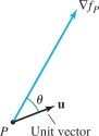
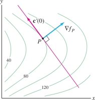
We are now in a position to draw some interesting and important conclusions about the gradient. First, suppose that \(\nabla f_P\ne \textbf{0}\) and let \({\bf{u}}\) be a unit vector (Figure 14.47). By the properties of the dot product, \begin{equation*} D_{{\bf{u}}}f(P) = \nabla f_P{\cdot}{\bf{u}} = \left \| {\nabla f_P} \right \|\cos\theta\tag{5} \end{equation*} where \(\theta\) is the angle between \(\nabla f_P\) and \({\bf{u}}\). In other words, the rate of change in a given direction varies with the cosine of the angle \(\theta\) between the gradient and the direction.
REMINDER
For any vectors \({\bf{u}}\) and \({\bf{v}}\), \[ {\bf{v}}{\cdot}{\bf{u}}=\left \| {\bf{v}} \right \|\left \| {\bf{u}} \right \|\cos\theta \] where \(\theta\) is the angle between \({\bf{v}}\) and \({\bf{u}}\). If \({\bf{u}}\) is a unit vector, then \[ {\bf{v}}{\cdot}{\bf{u}}=\left \| {\bf{v}} \right \| \cos\theta \]
Because the cosine takes values between \(-1\) and \(1\), we have \[ -\left \| {\nabla f_P} \right \|\le D_{{\bf{u}}}f(P)\le \left \| {\nabla f_P} \right \| \]
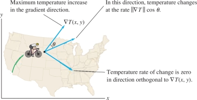
Since \(\cos 0 = 1\), the maximum value of \(D_{{\bf{u}}}f(P)\) occurs for \(\theta = 0 \)—that is, when \({\bf{u}}\) points in the direction of \(\nabla f_P\). In other words the gradient vector points in the direction of the maximum rate of increase, and this maximum rate is \(\left \| {\nabla f_P} \right \|\). Similarly, \(f\) decreases most rapidly in the opposite direction, \(-\nabla f_P\), because \(\cos\theta=-1\) for \(\theta=\pi\). The rate of maximum decrease is \(-\left \| {\nabla f_P} \right \|\). The directional derivative is zero in directions orthogonal to the gradient because \(\cos\frac{\pi}{2} = 0\).
In the earlier scenario where the biker Chloe rides along a path (Figure 14.48), the temperature \(T\) changes at a rate that depends on the cosine of the angle \(\theta\) between \(\nabla T\) and the direction of motion.
820
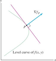
Another key property is that gradient vectors are normal to level curves (Figure 14.49). To prove this, suppose that \(P\) lies on the level curve \(f(x,y)=k\). We parametrize this level curve by a path \({\bf{c}}(t)\) such that \({\bf{c}}(0)=P\) and \({\bf{c}}'(0)\ne \mathbf{0}\) (this is possible whenever \(\nabla f_P\ne \mathbf{0}\)). Then \(f({\bf{c}}(t))=k\) for all \(t\), so by the Chain Rule, \[ \nabla f_P\cdot {\bf{c}}'(0) = \frac{d }{d t}f({\bf{c}}(t))\bigg|_{t=0}=\frac{d }{d t}k=0 \] This proves that \(\nabla f_P\) is orthogonal to \({\bf{c}}'(0)\), and since \({\bf{c}}'(0)\) is tangent to the level curve, we conclude that \(\nabla f_P\) is normal to the level curve (Figure 14.49). For functions of three variables, a similar argument shows that \(\nabla f_P\) is normal to the level surface \(f(x,y,z)=k\) through \(P\).
REMINDER
- The words “normal” and “orthogonal” both mean “perpendicular.”
- We say that a vector is normal to a curve at a point \(P\) if it is normal to the tangent line to the curve at \(P\).
THEOREM 4 Interpretation of the Gradient
Assume that \(\nabla f_P\ne {\bf{0}}\). Let \({\bf{u}}\) be a unit vector making an angle \(\theta\) with \(\nabla f_P\). Then \begin{equation*} \boxed{ D_{{\bf{u}}}f(P) = \left \| {\nabla f_P} \right \|\cos\theta}\tag{6} \end{equation*}
- \(\nabla f_P\) points in the direction of maximum rate of increase of \(f\) at \(P\).
- \(-\nabla f_P\) points in the direction of maximum rate of decrease at \(P\).
- \(\nabla f_P\) is normal to the level curve (or surface) of \(f\) at \(P\).
GRAPHICAL INSIGHT
At each point \(P\), there is a unique direction in which \(f(x,y)\) increases most rapidly (per unit distance). Theorem 4 tells us that this chosen direction is perpendicular to the level curves and that it is specified by the gradient vector (Figure 14.50). For most functions, however, the direction of maximum rate of increase varies from point to point.
EXAMPLE 8
Let \(f(x,y)=x^4y^{-2}\) and \(P=(2,1)\). Find the unit vector that points in the direction of maximum rate of increase at \(P\).
Solution The gradient points in the direction of maximum rate of increase, so we evaluate the gradient at \(P\): \[ \nabla f = \left\langle 4x^3y^{-2}, -2x^4y^{-3}\right\rangle,\qquad \nabla f_{(2,1)}=\left\langle 32,-32\right\rangle \]
The unit vector in this direction is \[ {\bf{u}} = \frac{\left\langle 32,-32\right\rangle}{\left \| {\left\langle 32,-32\right\rangle} \right \|} = \frac{\left\langle 32,-32\right\rangle}{32\sqrt{2}} = \left\langle \frac{\sqrt{2}}2,-\frac{\sqrt{2}}2\right\rangle \]
EXAMPLE 9
The altitude of a mountain at \((x,y)\) is \[ f(x,y)=2500 + 100(x + y^2)e^{-0.3y^2} \] where \(x, y\) are in units of 100 m.
- (a) Find the directional derivative of \(f\) at \(P=(-1,-1)\) in the direction of unit vector \({\bf{u}}\) making an angle of \(\theta = \frac{\pi}4\) with the gradient (Figure 14.51).
- (b) What is the interpretation of this derivative?
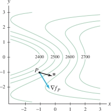
Solution First compute \(\left \| {\nabla f_P} \right \|\): \[ \begin{array}{rlrl} f_x(x,y) &= 100e^{-0.3 y^2},&\qquad f_y(x,y) & = 100y(2 - 0.6x - 0.6y^2)e^{-0.3 y^2}\\ f_x(-1,-1)&=100e^{-0.3} \approx 74, &\qquad f_y(-1,-1) &= -200 e^{-0.3} \approx -148 \end{array} \]
821
Hence, \(\nabla f_P \approx \left\langle 74 , -148 \right\rangle\) and \[ \left \| {\nabla f_P} \right \| \approx \sqrt{74^2+(-148)^2} \approx 165.5 \]
Apply Eq. (6) with \(\theta = \pi/4\): \[ D_{{\bf{u}}}f(P) = \left \| {\nabla f_P} \right \|\cos\theta \approx 165.5 \left(\frac{\sqrt{2}}{2}\right) \approx 117 \]
Recall that \(x\) and \(y\) are measured in units of 100 meters. Therefore, the interpretation is: If you stand on the mountain at the point lying above \((-1,-1)\) and begin climbing so that your horizontal displacement is in the direction of \({\bf{u}}\), then your altitude increases at a rate of 117 meters per 100 meters of horizontal displacement, or 1.17 meters per meter of horizontal displacement.
The symbol \(\psi\) (pronounced “p-sigh” or “p-see”) is the lowercase Greek letter psi.
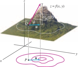
CONCEPTUAL INSIGHT
The directional derivative is related to the angle of inclination \(\psi\) in Figure 14.52. Think of the graph of \(z=f(x,y)\) as a mountain lying over the \(xy\)-plane. Let \(Q\) be the point on the mountain lying above a point \(P = (a,b)\) in the \(xy\)-plane. If you start moving up the mountain so that your horizontal displacement is in the direction of \({\bf{u}}\), then you will actually be moving up the mountain at an angle of inclination \(\psi\) defined by \begin{equation*} \tan\psi = D_{{\bf{u}}}f(P)\tag{7} \end{equation*}
The steepest direction up the mountain is the direction for which the horizontal displacement is in the direction of \(\nabla f_{P}\).
EXAMPLE 10 Angle of Inclination
You are standing on the side of a mountain in the shape \(z=f(x,y)\), at a point \(Q=(a,b,f(a,b))\), where \(\nabla f_{(a,b)} =\left\langle 0.4,0.02\right\rangle\). Find the angle of inclination in a direction making an angle of \(\theta = \frac{\pi}3\) with the gradient.
Solution The gradient has length \(\left \| {\nabla f_{(a,b)}} \right \| = \sqrt{(0.4)^2+(0.02)^2}\approx 0.4\). If \({\bf{u}}\) is a unit vector making an angle of \(\theta = \frac{\pi}3 \) with \(\nabla f_{(a,b)}\), then \[ D_{{\bf{u}}}f(a,b) = \left \| {\nabla f_{(a,b)}} \right \| \cos \frac{\pi}3 \approx (0.4)(0.5) = 0.2 \]
The angle of inclination at \(Q\) in the direction of \({\bf{u}}\) satisfies \(\tan\psi = 0.2\). It follows that \(\psi\approx \tan^{-1}0.2 \approx 0.197\) rad or approximately \(11.3^\circ\).
822
Another use of the gradient is in finding normal vectors on a surface with equation \(F(x,y,z)=k\), where \(k\) is a constant. Let \(P = (a,b,c)\) and assume that \(\nabla F_P\ne {\bf{0}}\). Then \(\nabla F_P\) is normal to the level surface \(F(x,y,z)=k\) by Theorem 4. The tangent plane at \(P\) has equation \[ \nabla F_P{\cdot}\left\langle x-a,y-b,z-c\right\rangle = 0 \]
Expanding the dot product, we obtain \[ \boxed{F_x(a,b,c)(x-a) + F_y(a,b,c)(y-b) + F_z(a,b,c)(z-c) = 0} \]
EXAMPLE 11 Normal Vector and Tangent Plane
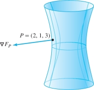
Find an equation of the tangent plane to the surface \(4x^2+9y^2-z^2=16\) at \(P = (2,1,3)\).
Solution Let \(F(x,y,z)=4x^2+9y^2-z^2\). Then \[ \nabla F = \left\langle 8x,18y,-2z \right\rangle,\qquad \nabla F_P=\nabla F_{(2,1,3)}=\left\langle 16,18,-6\right\rangle \]
The vector \(\left\langle 16,18,-6\right\rangle\) is normal to the surface \(F(x,y,z)=16\) (Figure 14.53), so the tangent plane at \(P\) has equation \[ 16(x-2)+18(y-1)-6(z-3)=0\qquad\textrm{or}\qquad 16x+18y-6z=32 \]
14.5.1 Summary
- The gradient of a function \(f\) is the vector of partial derivatives: \[ \nabla f = \left\langle \frac{\partial f}{\partial x},\frac{\partial f}{\partial y} \right\rangle \qquad\textrm{or}\qquad \nabla f = \left\langle \frac{\partial f}{\partial x},\frac{\partial f}{\partial y},\frac{\partial f}{\partial z} \right\rangle \]
- Chain Rule for Paths: \[ {\frac{d }{d t} f({\bf{c}}(t)) = \nabla f_{{\bf{c}}(t)}{\cdot} {\bf{c}}'(t)} \]
- Derivative of \(f\) with respect to \({\bf{v}} = \left\langle h, k\right\rangle\): \[ D_{{\bf{v}}}f(a,b) = \lim_{t\to 0}\frac{f(a+th,b+tk)-f(a,b)}t \] This definition extends to three or more variables.
- Formula for the derivative with respect to \({\bf{v}}\): \(D_{{\bf{v}}} f(a,b) = \nabla f_{(a,b)} \cdot {\bf{v}}\).
- For \({\bf{u}}\) a unit vector, \(D_{{\bf{u}}}f\) is called the directional derivative.
- – If \({\bf{u}}=\dfrac{{\bf{v}}}{\left \| {\bf{v}} \right \|}\), then \(D_{{\bf{u}}} f(a,b) = \dfrac1{\left \| {\bf{v}} \right \|}D_{{\bf{v}}} f(a,b)\).
- – \(D_{{\bf{u}}} f(a,b) = \left \| {\nabla f_{(a,b)}} \right \|\cos\theta\), where \(\theta\) is the angle between \(\nabla f_{(a,b)}\) and \({\bf{u}}\).
- Basic geometric properties of the gradient (assume \(\nabla f_P \neq {\bf{0}}\)):
- – \(\nabla f_P\) points in the direction of maximum rate of increase. The maximum rate of increase is \(\left \| {\nabla f_P} \right \|\).
- – \(-\nabla f_P\) points in the direction of maximum rate of decrease. The maximum rate of decrease is \(-\left \| {\nabla f_P} \right \|\).
- – \(\nabla f_P\) is orthogonal to the level curve (or surface) through \(P\).
- Equation of the tangent plane to the level surface \(F(x,y,z)=k\) at \(P=(a,b,c)\): \[ \begin{array}{c} \displaystyle \nabla F_P{\cdot}\left\langle x-a,y-b,z-c\right\rangle=0\\ \displaystyle F_x(a,b,c)(x-a) + F_y(a,b,c)(y-b) + F_z(a,b,c)(z-c)=0 \end{array} \]
823