14.7 Optimization in Several Variables
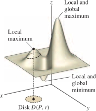
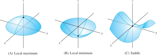
Recall that optimization is the process of finding the extreme values of a function. This amounts to finding the highest and lowest points on the graph over a given domain. As we saw in the one-variable case, it is important to distinguish between local and global extreme values. A local extreme value is a value \(f(a,b)\) that is a maximum or minimum in some small open disk around \((a,b)\) (Figure 14.56).
DEFINITION Local Extreme Values
A function \(f(x,y)\) has a local extremum at \(P=(a,b)\) if there exists an open disk \(D(P,r)\) such that:
- Local maximum: \(f(x,y)\le f(a,b)\) for all \((x,y)\in D(P,r)\)
- Local minimum: \(f(x,y)\ge f(a,b)\) for all \((x,y)\in D(P,r)\)
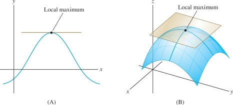
Fermat’s Theorem states that if \(f(a)\) is a local extreme value, then \(a\) is a critical point and thus the tangent line (if it exists) is horizontal at \(x=a\). We can expect a similar result for functions of two variables, but in this case, it is the tangent plane that must be horizontal (Figure 14.57). The tangent plane to \(z=f(x,y)\) at \(P = (a,b)\) has equation \[ z = f(a,b) + f_x(a,b)(x-a)+ f_y(a,b)(y-b) \]
REMINDER
The term “extremum” (the plural is “extrema”) means a minimum or maximum value.
Thus, the tangent plane is horizontal if \(f_x(a,b) = f_y(a,b) =0\)—that is, if the equation reduces to \(z=f(a,b)\). This leads to the following definition of a critical point, where we take into account the possibility that one or both partial derivatives do not exist.
834
DEFINITION Critical Point
A point \(P = (a,b)\) in the domain of \(f(x,y)\) is called a critical point if:
- \(f_x(a,b) =0\) or \(f_x(a,b)\) does not exist, and
- \(f_y(a,b)=0\) or \(f_y(a,b)\) does not exist.
- More generally, \((a_1,\dots,a_n)\) is a critical point of \(f(x_1,\dots,x_n)\) if each partial derivative satisfies \[ f_{x_j}(a_1,\dots,a_n) = 0 \] or does not exist.
- Theorem 1 holds in any number of variables: Local extrema occur at critical points.
As in the single-variable case, we have
THEOREM 1 Fermat’s Theorem
If \(f(x,y)\) has a local minimum or maximum at \(P=(a,b)\), then \((a,b)\) is a critical point of \(f(x,y)\).
proof If \(f(x,y)\) has a local minimum at \(P=(a,b)\), then \( f(x,y)\ge f(a,b)\) for all \((x,y)\) near \((a,b)\). In particular, there exists \(r>0\) such that \(f(x,b)\ge f(a,b)\) if \(|x-a|<r\). In other words, \(g(x)=f(x,b)\) has a local minimum at \(x=a\). By Fermat’s Theorem for functions of one variable, either \(g'(a)=0\) or \(g'(a)\) does not exist. Since \(g'(a) = f_x(a,b)\), we conclude that either \(f_x(a,b)=0\) or \(f_x(a,b)\) does not exist. Similarly, \(f_y(a,b)=0\) or \(f_y(a,b)\) does not exist. Therefore, \(P=(a,b)\) is a critical point. The case of a local maximum is similar.
Usually, we deal with functions whose partial derivatives exist. In this case, finding the critical points amounts to solving the simultaneous equations \(f_x(x,y)=0\) and \(f_y(x,y)=0\).
EXAMPLE 1
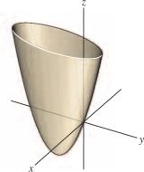
Show that \(f(x,y) = 11x^2 - 2xy + 2y^2 + 3y\) has one critical point. Use Figure 14.58 to determine whether it corresponds to a local minimum or maximum.
Solution Set the partial derivatives equal to zero and solve: \[ \begin{array}{rl} f_x(x,y) &= 22x-2y=0\\ f_y(x,y) &= -2x+4y+3=0 \end{array} \]
By the first equation, \(y=11x\). Substituting \(y=11x\) in the second equation gives \[ -2x+4y+3 = -2x+4(11x)+3 = 42x+3=0 \]
Thus \(x = -\frac1{14}\) and \(y=-\frac{11}{14}\). There is just one critical point, \(P=\big(-\frac1{14},-\frac{11}{14}\big)\). Figure 14.58 shows that \(f(x,y)\) has a local minimum at \(P\).
It is not always possible to find the solutions exactly, but we can use a computer to find numerical approximations.
EXAMPLE 2 Numerical Example
![]() Use a computer algebra system to approximate the critical points of
\[
f(x,y) = \frac{x-y}{2x^2+8y^2+3}
\]
Use a computer algebra system to approximate the critical points of
\[
f(x,y) = \frac{x-y}{2x^2+8y^2+3}
\]
Are they local minima or maxima? Refer to Figure 14.59.
Solution We use a CAS to compute the partial derivatives and solve \[ \begin{array}{rl} f_x(x,y) &=\frac{-2x^2+8y^2+4xy+3}{(2x^2+8y^2+3)^2}=0\\ f_y(x,y) &=\frac{-2x^2+8y^2-16xy-3 }{(2x^2+8y^2+3)^2} =0 \end{array} \]
835
To solve these equations, set the numerators equal to zero. Figure 14.59 suggests that \(f(x,y)\) has a local max with \(x>0\) and a local min with \(x<0\). The following Mathematica command searches for a solution near \((1,0)\):
FindRoot[{-2x^2+8y^2+4xy+3 == 0, -2x^2+8y^2-16xy-3 == 0},
{{x,1},{y,0}}]
The result is
{x -> 1.095, y -> -0.274}
Thus, \((1.095, -0.274)\) is an approximate critical point where, by Figure 14.59, \(f\) takes on a local maximum. A second search near \((-1,0)\) yields \((-1.095,0.274)\), which approximates the critical point where \(f(x,y)\) takes on a local minimum.
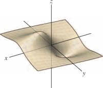
We know that in one variable, a function \(f(x)\) may have a point of inflection rather than a local extremum at a critical point. A similar phenomenon occurs in several variables. Each of the functions in Figure 14.60 has a critical point at \((0,0)\). However, the function in Figure 14.60 has a saddle point, which is neither a local minimum nor a local maximum. If you stand at the saddle point and begin walking, some directions take you uphill and other directions take you downhill.
As in the one-variable case, there is a Second Derivative Test for determining the type of a critical point \((a,b)\) of a function \(f(x,y)\) in two variables. This test relies on the sign of the discriminant \(D = D(a,b)\), defined as follows: \[ \boxed{ D = D(a,b) = f_{xx}(a,b)f_{yy}(a,b)-f_{xy}^2(a,b)} \]
The discriminant is also referred to as the “Hessian determinant.”
THEOREM 2 Second Derivative Test
Let \(P=(a,b)\) be a critical point of \(f(x,y)\). Assume that \(f_{xx}, f_{yy}, f_{xy}\) are continuous near \(P\). Then:
- (i) If \(D>0\) and \(f_{xx}(a,b)>0\), then \(f(a,b)\) is a local minimum.
- (ii) If \(D>0\) and \(f_{xx}(a,b)<0\), then \(f(a,b)\) is a local maximum.
- (iii) If \(D<0\), then \(f\) has a saddle point at \((a,b)\).
- (iv) If \(D=0\), the test is inconclusive.
If \(D>0\), then \(f_{xx}(a,b)\) and \(f_{yy}(a,b)\) must have the same sign, so the sign of \(f_{yy}(a,b)\) also determines whether \(f(a,b)\) is a local minimum or a local maximum.
A proof of this theorem is discussed at the end of this section.
836
EXAMPLE 3 Applying the Second Derivative Test
Find the critical points of \[ f(x,y) = (x^2+y^2)e^{-x} \] and analyze them using the Second Derivative Test.
Solution
Step 1. Find the critical points.
Set the partial derivatives equal to zero and solve: \[ \begin{array}{rl} f_x(x,y) &= -(x^2+y^2)e^{-x}+2xe^{-x}= (2x - x^2 - y^2)e^{-x} = 0\\ f_y(x,y) &= 2ye^{-x} = 0\quad \Rightarrow\quad y=0 \end{array} \]
Substituting \(y=0\) in the first equation then gives \[ (2x - x^2 - y^2)e^{-x} = (2x - x^2)e^{-x} = 0\quad\Rightarrow\quad x=0, 2 \]
The critical points are \((0,0)\) and \((2,0)\) [Figure 14.61].

Step 2. Compute the second-order partials.
\[ \begin{array}{rl} f_{xx}(x,y) &=\frac{\partial }{\partial x} \big((2x - x^2-y^2)e^{-x}\big) =(2-4x+x^2+y^2)e^{-x}\\ f_{yy}(x,y) &=\frac{\partial }{\partial y}(2ye^{-x}) = 2e^{-x}\\ f_{xy}(x,y) &=f_{yx}(x,y)=\frac{\partial }{\partial x} (2ye^{-x}) = -2ye^{-x}\\ \end{array} \]
Step 3. Apply the Second Derivative Test.
| Critical Point | \(f_{xx}\) | \(f_{yy}\) | \(f_{xy}\) | Discriminant \(D = f_{xx}f_{yy}-f_{xy}^2\) | Type |
|---|---|---|---|---|---|
| \((0,0)\) | 2 | 2 | 0 | \(2(2)-0^2=4\) | Local minimum since \(D>0\) and \(f_{xx}>0\) |
| \((2,0)\) | \(-2e^{-2}\) | \(2e^{-2}\) | 0 | \(-2e^{-2}(2e^{-2}) - 0^2 = -4e^{-4}\) | Saddle since \(D<0\) |
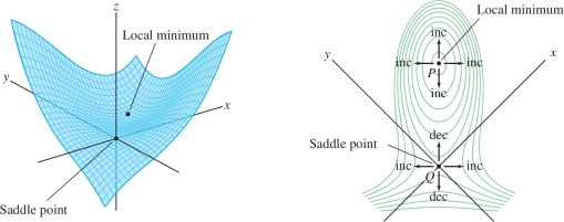
GRAPHICAL INSIGHT
We can also read off the type of critical point from the contour map. Notice that the level curves in Figure 14.62 encircle the local minimum at \(P\), with \(f\) increasing in all directions emanating from \(P\). By contrast, \(f\) has a saddle point at \(Q\): The neighborhood near \(Q\) is divided into four regions in which \(f(x,y)\) alternately increases and decreases.
837
EXAMPLE 4
Analyze the critical points of \(f(x,y) = x^3 + y^3 - 12xy\).
Solution Again, we set the partial derivatives equal to zero and solve: \[ \begin{array}{rl} f_x(x,y) &= 3x^2-12y=0\quad\Rightarrow \quad y = \frac14x^2\\ f_y(x,y) &= 3y^2-12x=0 \end{array} \]
Substituting \(y=\frac14x^2\) in the second equation yields \[ 3y^2-12x = 3\left(\frac14x^2\right)^2 - 12x = \frac3{16}x(x^3-64) = 0\quad\Rightarrow \quad x=0, 4 \]
Since \(y=\frac14x^2\), the critical points are \((0,0)\) and \((4,4)\).
We have \[ f_{xx}(x,y)=6x,\qquad f_{yy}(x,y)=6y,\qquad f_{xy}(x,y)=-12 \]
The Second Derivative Test confirms what we see in Figure 14.62: \(f\) has a local min at \((4,4)\) and a saddle at \((0,0)\).
| Critical Point | \(f_{xx}\) | \(f_{yy}\) | \(f_{xy}\) | Discriminant \(D = f_{xx}f_{yy}-f_{xy}^2\) | Type |
|---|---|---|---|---|---|
| \((0,0)\) | 0 | 0 | \(-12\) | \(0(0)-12^2=-144\) | Saddle since \(D<0\) |
| \((4,4)\) | 24 | 24 | \(-12\) | \(24(24) - 12^2 = 432\) | Local minimum since \(D>0\) and \(f_{xx}>0\) |
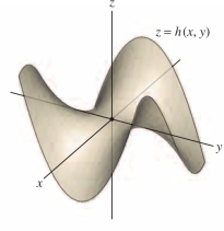
GRAPHICAL INSIGHT
A graph can take on a variety of different shapes at a saddle point. The graph of \(h(x,y)\) in Figure 14.63 is called a “monkey saddle” (because a monkey can sit on this saddle with room for his tail in the back).
Global Extrema
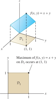
Often we are interested in finding the minimum or maximum value of a function \(f\) on a given domain \({\mathcal{D}}\). These are called global or absolute extreme values. However, global extrema do not always exist. The function \(f(x,y)=x+y\) has a maximum value on the unit square \({\mathcal{D}}_1\) in Figure 14.64 (the max is \(f(1,1)=2\)), but it has no maximum value on the entire plane \({\bf{R}}^2\).
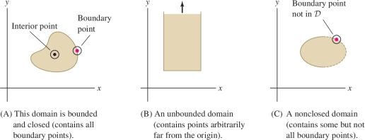
To state conditions that guarantee the existence of global extrema, we need a few definitions. First, we say that a domain \({\mathcal{D}}\) is bounded if there is a number \(M>0\) such that \({\mathcal{D}}\) is contained in a disk of radius \(M\) centered at the origin. In other words, no point of \({\mathcal{D}}\) is more than a distance \(M\) from the origin [Figures 11(A) and 11(B)]. Next, a point \(P\) is called:
- An interior point of \({\mathcal{D}}\) if \({\mathcal{D}}\) contains some open disk \(D(P,r)\) centered at \(P\).
- A boundary point of \({\mathcal{D}}\) if every disk centered at \(P\) contains points in \({\mathcal{D}}\) and points not in \({\mathcal{D}}\).
CONCEPTUAL INSIGHT
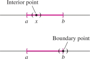
To understand the concept of interior and boundary points, think of the familiar case of an interval \(I = [a,b]\) in the real line \({\bf{R}}\) (Figure 14.65). Every point \(x\) in the open interval \((a,b)\) is an interior point of \(I\) (because there exists a small open interval around \(x\) entirely contained in \(I\)). The two endpoints \(a\) and \(b\) are boundary points (because every open interval containing \(a\) or \(b\) also contains points not in \(I\)).
838
The interior of \({\mathcal{D}}\) is the set of all interior points, and the boundary of \({\mathcal{D}}\) is the set of all boundary points. In Figure 14.66, the boundary is the curve surrounding the domain. The interior consists of all points in the domain not lying on the boundary curve.
A domain \({\mathcal{D}}\) is called closed if \({\mathcal{D}}\) contains all its boundary points (like a closed interval in \({\bf{R}}\)). A domain \({\mathcal{D}}\) is called open if every point of \({\mathcal{D}}\) is an interior point (like an open interval in \({\bf{R}}\)). The domain in Figure 14.66 is closed because the domain includes its boundary curve. In Figure 14.66, some boundary points are included and some are excluded, so the domain is neither open nor closed.
In Section 4.2, we stated two basic results. First, a continuous function \(f(x)\) on a closed, bounded interval \([a,b]\) takes on both a minimum and a maximum value on \([a,b]\). Second, these extreme values occur either at critical points in the interior \((a,b)\) or at the endpoints. Analogous results are valid in several variables.
THEOREM 3 Existence and Location of Global Extrema
Let \(f(x,y)\) be a continuous function on a closed, bounded domain \({\mathcal{D}}\) in \({\bf{R}}^2\). Then:
- (i) \(f(x,y)\) takes on both a minimum and a maximum value on \({\mathcal{D}}\).
- (ii) The extreme values occur either at critical points in the interior of \({\mathcal{D}}\) or at points on the boundary of \({\mathcal{D}}\).
EXAMPLE 5
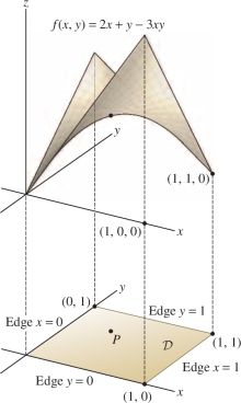
Find the maximum value of \(f(x,y)=2x+y-3xy\) on the unit square \({\mathcal{D}} = \{(x,y) : 0 \leq x, y \leq 1\}\).
Solution By Theorem 3, the maximum occurs either at a critical point or on the boundary of the square (Figure 14.67).
Step 1. Examine the critical points.
Set the partial derivatives equal to zero and solve: \[ \begin{array}{rl} f_x(x,y) &= 2-3y = 0\quad\Rightarrow\quad y=\frac23,\qquad f_y(x,y) = 1-3x = 0\quad \Rightarrow\quad x = \frac13 \end{array} \]
There is a unique critical point \(P=\big(\frac13,\frac23\big)\) and \[ f(P)=f\left(\frac13,\frac23\right)= 2\left(\frac13\right)+\left(\frac23\right)-3\left(\frac13\right)\left(\frac23\right) = \frac23 \]
Step 2. Check the boundary.
We do this by checking each of the four edges of the square separately. The bottom edge is described by \(y=0\), \(0\le x \le 1\). On this edge, \(f(x,0)= 2x\), and the maximum value occurs at \(x=1\), where \(f(1,0)=2\). Proceeding in a similar fashion with the other edges, we obtain
839
| Edge | Restriction of \(f(x,y)\) to Edge | Maximum of \(f(x,y)\) on Edge |
|---|---|---|
| Lower: \(y=0\), \(0\le x \le 1\) | \(f(x,0)= 2x\) | \(f(1,0)=2\) |
| Upper: \(y=1\), \(0\le x \le 1\) | \(f(x,1)=1-x\) | \(f(0,1)=1\) |
| Left: \(x=0\), \(0\le y \le 1\) | \(f(0,y)=y\) | \(f(0,1)=1\) |
| Right: \(x=1\), \(0\le y \le 1\) | \(f(1,y)=2-2y\) | \(f(1,0)=2\) |
Step 3. Compare.
The maximum of \(f\) on the boundary is \(f(1,0)=2\). This is larger than the value \(f(P)= \frac23\) at the critical point, so the maximum of \(f\) on the unit square is 2.
EXAMPLE 6 Box of Maximum Volume
Find the maximum volume of a box inscribed in the tetrahedron bounded by the coordinate planes and the plane \(\tfrac13x +y+z=1\).
Solution
Step 1. Find a function to be maximized.
Let \(P=(x,y,z)\) be the corner of the box lying on the front face of the tetrahedron (Figure 14.68). Then the box has sides of lengths \(x, y, z\) and volume \(V = xyz\). Using \(\frac13x+y+z=1\), or \(z = 1-\frac13x-y\), we express \(V\) in terms of \(x\) and \(y\): \[ V(x,y) = xyz = xy\left(1-\frac13x-y\right) = xy - \frac13x^2y-xy^2 \]
Our problem is to maximize \(V\), but which domain \({\mathcal{D}}\) should we choose? We let \({\mathcal{D}}\) be the shaded triangle \(\triangle\) OAB in the \(xy\)-plane in Figure 14.68. Then the corner point \(P=(x,y,z)\) of each possible box lies above a point \((x,y)\) in \({\mathcal{D}}\). Because \({\mathcal{D}}\) is closed and bounded, the maximum occurs at a critical point inside \({\mathcal{D}}\) or on the boundary of \({\mathcal{D}}\).

Step 2. Examine the critical points.
First, set the partial derivatives equal to zero and solve: \[ \begin{array}{rl} \frac{\partial V}{\partial x} &= y - \frac23xy-y^2 = y\left(1 - \frac23x - y\right) = 0\\ \frac{\partial V}{\partial y} &= x - \frac13x^2-2xy = x\left(1 - \frac13x - 2y\right) =0 \end{array} \]
If \(x=0\) or \(y=0\), then \((x,y)\) lies on the boundary of \({\mathcal{D}}\), so assume that \(x\) and \(y\) are both nonzero. Then the first equation gives us \[ \begin{array}{rl} 1 - \frac23x - y &= 0\quad\Rightarrow\quad y=1-\frac23x \end{array} \]
The second equation yields \[ 1 - \frac13x - 2y = 1-\frac13x-2\left(1-\frac23x\right)=0\quad\Rightarrow\quad x-1=0 \quad\Rightarrow\quad x=1 \]
For \(x=1\), we have \(y=1-\frac23x = \frac13\). Therefore, \(\big(1,\frac13\big)\) is a critical point, and \[ V\left(1,\frac13\right) =(1)\frac13-\frac13(1)^2\frac13-(1)\left(\frac13\right)^2 = \frac19 \]
Step 3. Check the boundary.
We have \(V(x,y)=0\) for all points on the boundary of \({\mathcal{D}}\) (because the three edges of the boundary are defined by \(x=0\), \(y=0\), and \(1-\frac13x-y=0\)). Clearly, then, the maximum occurs at the critical point, and the maximum volume is \(\frac19\).
840
Proof of the Second Derivative Test The proof is based on “completing the square” for quadratic forms. A quadratic form is a function \[ \boxed{Q(h,k) = ah^2+2bhk+ck^2} \] where \(a, b, c\) are constants (not all zero). The discriminant of \(Q\) is the quantity \[ \boxed{D=ac-b^2} \]
Some quadratic forms take on only positive values for \((h,k) \ne (0,0)\), and others take on both positive and negative values. According to the next theorem, the sign of the discriminant determines which of these two possibilities occurs.
To illustrate Theorem 4, consider \[ Q(h,k) = h^2+2hk+2k^2 \] It has a positive discriminant \[ D = (1)(2)-1= 1 \] We can see directly that \(Q(h,k)\) takes on only positive values for \((h,k)\ne (0,0)\) by writing \(Q(h,k)\) as \[ Q(h,k) = (h+k)^2+k^2 \]
THEOREM 4
With \(Q(h,k)\) and \(D\) as above:
- (i) If \(D>0\) and \(a>0\), then \(Q(h,k)>0\) for \((h,k)\ne (0,0)\).
- (ii) If \(D>0\) and \(a<0\), then \(Q(h,k)<0\) for \((h,k)\ne (0,0)\).
- (iii) If \(D<0\), then \(Q(h,k)\) takes on both positive and negative values.
proof Assume first that \(a\ne 0\) and rewrite \(Q(h,k)\) by “completing the square”: \begin{equation*} \begin{array}{rcl} Q(h,k) &=& ah^2+2bhk+ck^2 = a\left(h+\frac{b}{a}k\right)^2 + \left(c-\frac{b^2}{a}\right)k^2\\ &=& a\left(h+\frac{b}{a}k\right)^2 + \frac{D}{a} k^2 \end{array}\tag{1} \end{equation*}
If \(D>0\) and \(a>0\), then \(D/a>0\) and both terms in Eq. (1) are nonnegative. Furthermore, if \(Q(h,k)=0\), then each term in Eq. (1) must equal zero. Thus \(k=0\) and \(h+\tfrac{b}{a}k=0\), and then, necessarily, \(h=0\). This shows that \(Q(h,k)> 0\) if \((h,k)\ne 0\), and (i) is proved. Part (ii) follows similarly. To prove (iii), note that if \(a\ne 0\) and \(D<0\), then the coefficients of the squared terms in Eq. (1) have opposite signs and \(Q(h,k)\) takes on both positive and negative values. Finally, if \(a = 0\) and \(D < 0\), then \(Q(h,k) = 2bhk + ck^2\) with \(b\neq 0\). In this case, \(Q(h,k)\) again takes on both positive and negative values.
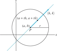
Now assume that \(f(x,y)\) has a critical point at \(P=(a,b)\). We shall analyze \(f\) by considering the restriction of \(f(x,y)\) to the line (Figure 14.69) through \(P=(a,b)\) in the direction of a unit vector \(\left\langle h,k\right\rangle\): \[ F(t) = f(a+th,b+tk) \]
Then \(F(0) = f(a,b)\). By the Chain Rule, \[ F'(t)= f_x(a+th,b+tk)h+f_y(a+th,b+tk)k \]
Because \(P\) is a critical point, we have \(f_x(a,b) = f_y(a,b) = 0\), and therefore, \[ F'(0) = f_x(a,b)h+f_y(a,b)k = 0 \]
Thus \(t=0\) is a critical point of \(F(t)\).
841
Now apply the Chain Rule again: \begin{equation*} \begin{array}{rcl} F''(t)&=& \frac{d }{d t}\Big(f_x(a+th,b+tk)h+f_y(a+th,b+tk)k\Big)\\ &=& \Big(f_{xx}(a+th,b+tk)h^2 + f_{xy}(a+th,b+tk)hk\Big)\\ &&\,\qquad\qquad\qquad\qquad\quad + \Big(f_{yx}(a+th,b+tk)kh + f_{yy}(a+th,b+tk)k^2\Big)\\ &=& f_{xx}(a+th,b+tk)h^2 + 2f_{xy}(a+th,b+tk)hk + f_{yy}(a+th,b+tk)k^2 \end{array}\tag{2} \end{equation*}
We see that \(F''(t)\) is the value at \((h,k)\) of a quadratic form whose discriminant is equal to \(D(a+th,b+tk)\). Here, we set \[ D(r,s)=f_{xx}(r,s)f_{yy}(r,s)-f_{xy}(r,s)^2 \]
Note that the discriminant of \(f(x,y)\) at the critical point \(P = (a,b)\) is \(D=D(a,b)\).
Case 1: \(D(a,b) > 0\) and \(f_{xx}(a,b)>0\). We must prove that \(f(a,b)\) is a local minimum. Consider a small disk of radius \(r\) around \(P\) (Figure 14.69). Because the second derivatives are continuous near \(P\), we can choose \(r>0\) so that for every unit vector \(\left\langle h,k\right\rangle\), \[ \begin{matrix} D(a+th,b+tk)>0 &\textrm{for }|t|<r\\ f_{xx}(a+th,b+tk)>0 &\textrm{for }|t|<r \end{matrix} \]
Then \(F''(t)\) is positive for \(|t|<r\) by Theorem 4(i). This tells us that \(F(t)\) is concave up, and hence \(F(0)<F(t)\) if \(0<|t|<|r|\) (see Exercise 64 in Section 4.4). Because \(F(0) = f(a,b)\), we may conclude that \(f(a,b)\) is the minimum value of \(f\) along each segment of radius \(r\) through \((a,b)\). Therefore, \(f(a,b)\) is a local minimum value of \(f\) as claimed. The case that \(D(a,b)>0\) and \(f_{xx}(a,b)<0\) is similar.
Case 2: \(D(a,b)<0\). For \(t=0\), Eq. (2) yields \[ F''(0) = f_{xx}(a,b)h^2 + 2f_{xy}(a,b)hk + f_{yy}(a,b)k^2 \]
Since \(D(a,b)<0\), this quadratic form takes on both positive and negative values by Theorem 4(iii). Choose \(\left\langle h, k\right\rangle\) for which \(F''(0)>0\). By the Second Derivative Test in one variable, \(F(0)\) is a local minimum of \(F(t)\), and hence, there is a value \(r>0\) such that \(F(0)<F(t)\) for all \(0<|t|<r\). But we can also choose \(\left\langle h, k\right\rangle\) so that \(F''(0)<0\), in which case \(F(0) >F(t)\) for \(0<|t|<r\) for some \(r>0\). Because \(F(0) = f(a,b)\), we conclude that \(f(a,b)\) is a local min in some directions and a local max in other directions. Therefore, \(f\) has a saddle point at \(P=(a,b)\).
14.7.1 Summary
- We say that \(P=(a,b)\) is a critical point of \(f(x,y)\) if
- – \(f_x(a,b) =0\) or \(f_x(a,b)\) does not exist, and
- – \(f_y(a,b)=0\) or \(f_y(a,b)\) does not exist.
- The local minimum or maximum values of \(f\) occur at critical points.
- The discriminant of \(f(x,y)\) at \(P = (a,b)\) is the quantity \[ D(a,b) = f_{xx}(a,b)f_{yy}(a,b) - f_{xy}^2(a,b) \]
- Second Derivative Test: If \(P=(a,b)\) is a critical point of \(f(x,y)\), then \[ \begin{array}{rl} D(a,b)>0, \,\,\,f_{xx}(a,b)>0 &\quad\Rightarrow\quad f(a,b)\textrm{ is a local minimum}\\[4pt] D(a,b)>0, \,\,\, f_{xx}(a,b)<0 &\quad\Rightarrow\quad f(a,b)\textrm{ is a local maximum}\\[4pt] D(a,b)<0 &\quad\Rightarrow\quad \textrm{saddle point}\\[4pt] D(a,b)=0 &\quad\Rightarrow\quad \textrm{test inconclusive} \end{array} \]
- A point \(P\) is an interior point of a domain \({\mathcal{D}}\) if \({\mathcal{D}}\) contains some open disk \(D(P,r)\) centered at \(P\). A point \(P\) is a boundary point of \({\mathcal{D}}\) if every open disk \(D(P,r)\) contains points in \({\mathcal{D}}\) and points not in \({\mathcal{D}}\). The interior of \({\mathcal{D}}\) is the set of all interior points, and the boundary is the set of all boundary points. A domain is closed if it contains all of its boundary points and open if it is equal to its interior.
- Existence and location of global extrema: If \(f\) is continuous and \({\mathcal{D}}\) is closed and bounded, then
- – \(f\) takes on both a minimum and a maximum value on \({\mathcal{D}}\).
- – The extreme values occur either at critical points in the interior of \({\mathcal{D}}\) or at points on the boundary of \({\mathcal{D}}\).
842