15.1 Integration in Two Variables
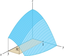
The integral of a function of two variables \(f(x,y)\), called a double integral, is denoted \[ \iint_{{\mathcal{D}}} f(x,y)\,dA \]
It represents the signed volume of the solid region between the graph of \(f(x,y)\) and a domain \({\mathcal{D}}\) in the \(xy\)-plane (Figure 15.1), where the volume is positive for regions above the \(xy\)-plane and negative for regions below.
There are many similarities between double integrals and the single integrals:
- Double integrals are defined as limits of sums.
- Double integrals are evaluated using the Fundamental Theorem of Calculus (but we have to use it twice—see the discussion of iterated integrals below).
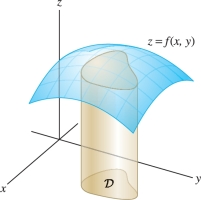
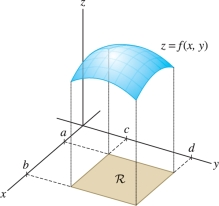
An important difference, however, is that the domain of integration plays a more prominent role in the multivariable case. In one variable, the domain of integration is simply an interval \([a,b]\). In two variables, the domain \({\mathcal{D}}\) is a plane region whose boundary may be curved (Figure 15.2).
In this section, we focus on the simplest case where the domain is a rectangle, leaving more general domains for Section 15.2. Let \[ {\mathcal{R}} = [a,b]\times[c,d] \] denote the rectangle in the plane (Figure 15.2) consisting of all points \((x,y)\) such that \[ {\mathcal{R}}{:}\quad a\le x \le b,\qquad c\le y\le d \]
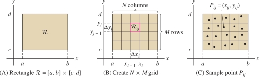
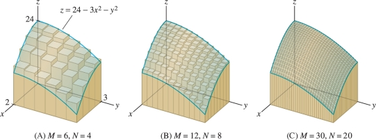
Like integrals in one variable, double integrals are defined through a three-step process: subdivision, summation, and passage to the limit. Figure 15.3 illustrates how the rectangle \({\mathcal{R}}\) is subdivided:
- 1. Subdivide \([a,b]\) and \([c,d]\) by choosing partitions: \[ a=x_0 < x_1 < \cdots < x_N=b, \qquad c=y_0 < y_1 < \cdots < y_M=d \] where \(N\) and \(M\) are positive integers.
- 2. Create an \(N\times M\) grid of subrectangles \({\mathcal{R}}_{ij}\).
- 3. Choose a sample point \(P_{ij}\) in each \({\mathcal{R}}_{ij}\).
861
Note that \({\mathcal{R}}_{ij}=[x_{i-1},x_i]\times[y_{j-1},y_j]\), so \({\mathcal{R}}_{ij}\) has area \[ \Delta A_{ij} =\Delta x_i\,\Delta y_j \] where \(\Delta x_i=x_i-x_{i-1}\) and \(\Delta y_j=y_j-y_{j-1}\).
Keep in mind that a Riemann sum depends on the choice of partition and sample points. It would be more proper to write \[ S_{N,M}(\{P_{ij}\},\{x_i\}, \{y_j\}) \] but we write \(S_{N,M}\) to keep the notation simple.
Next, we form the Riemann sum with the function values \(f(P_{ij})\): \[ S_{N,M} = \sum_{i=1}^N\sum_{j=1}^M f(P_{ij})\,\Delta A_{ij} = \sum_{i=1}^N\sum_{j=1}^M f(P_{ij})\,\Delta x_i\,\Delta y_j \]
The double summation runs over all \(i\) and \(j\) in the ranges \(1\le i \le N\) and \(1\le j \le M\), a total of \(NM\) terms.
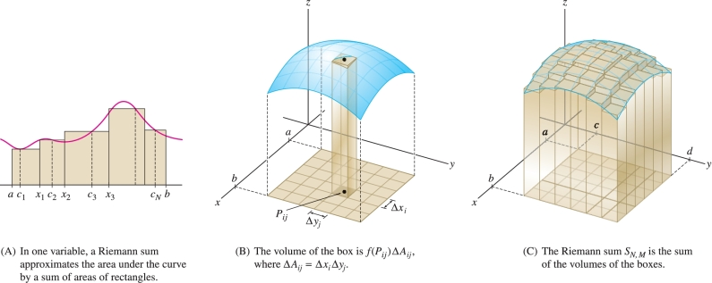
The geometric interpretation of \(S_{N,M}\) is shown in Figure 15.4. Each individual term \(f(P_{ij})\,\Delta A_{ij}\) of the sum is equal to the signed volume of the narrow box of height \(f(P_{ij})\) above \({\mathcal{R}}_{ij}\): \[ f(P_{ij})\,\Delta A_{ij} = f(P_{ij})\,\Delta x_i\,\Delta y_j = \underbrace{\textrm{height}\times\textrm{area}}_{\textrm{Signed volume of box}} \]
When \(f(P_{ij})\) is negative, the box lies below the \(xy\)-plane and has negative signed volume. The sum \(S_{N,M}\) of the signed volumes of these narrow boxes approximates volume in the same way that Riemann sums in one variable approximate area by rectangles [Figure 15.4].
862
The final step in defining the double integral is passing to the limit. We write \({\mathcal{P}}=\{\{x_i\},\{y_j\}\}\) for the partition and \(\left \| {{\mathcal{P}}} \right \|\) for the maximum of the widths \(\Delta x_i\), \(\Delta y_j\). As \(\left \| {{\mathcal{P}}} \right \|\) tends to zero (and both \(M\) and \(N\) tend to infinity), the boxes approximate the solid region under the graph more and more closely Figure 15.5. Here is the precise definition of the limit:
Limit of Riemann Sums
The Riemann sum \(S_{N,M}\) approaches a limit \(L\) as \(\left \| {{\mathcal{P}}} \right \| \to 0\) if, for all \(\epsilon > 0\), there exists \(\delta>0\) such that \[ |L - S_{N,M}| < \epsilon \] for all partitions satisfying \(\left \| {{\mathcal{P}}} \right \|<\delta\) and all choices of sample points.
In this case, we write \[ \lim_{\left \| {{\mathcal{P}}} \right \| \to 0} S_{N,M} = \lim_{\left \| {{\mathcal{P}}} \right \| \to 0} \sum_{i=1}^N\sum_{j=1}^M f(P_{ij})\,\Delta A_{ij} = L \]
This limit \(L\), if it exists, is the double integral \(\iint_{{\mathcal{R}}\,} f(x,y)\,dA\).
DEFINITION Double Integral over a Rectangle
The double integral of \(f(x,y)\) over a rectangle \({\mathcal{R}}\) is defined as the limit \[ \iint_{{\mathcal{R}}\,} f(x,y)\,dA = \lim_{\left \| {{\mathcal{P}}} \right \| \to 0} \sum_{i=1}^N\sum_{j=1}^M f(P_{ij})\Delta A_{ij} \]
If this limit exists, we say that \(f(x,y)\) is integrable over \({\mathcal{R}}\).
The double integral enables us to define the volume \(V\) of the solid region between the graph of a positive function \(f(x,y)\) and the rectangle \({\mathcal{R}}\) by \[ V = \iint_{{\mathcal{R}}\,} f(x,y)\,dA \]
If \(f(x,y)\) takes on both positive and negative values, the double integral defines the signed volume Figure 15.6.
863
In computations, we often assume that the partition \({\mathcal{P}}\) is regular, meaning that the intervals \([a,b]\) and \([c,d]\) are both divided into subintervals of equal length. In other words, the partition is regular if \(\Delta x_i=\Delta x\) and \(\Delta y_j=\Delta y\), where \[ \Delta x = \frac{b-a}N,\qquad \Delta y=\frac{d-c}M \]
For a regular partition, \(\left \| {{\mathcal{P}}} \right \|\) tends to zero as \(N\) and \(M\) tend to \(\infty\).
EXAMPLE 1 Estimating a Double Integral
Let \({\mathcal{R}} = [1,2.5]\times [1,2]\). Calculate \(S_{3,2}\) for the integral Figure 15.7 \[ \iint_{{\mathcal{R}}\,} xy\,dA \] using the following two choices of sample points:
- (a) Lower-left vertex
- (b) Midpoint of rectangle
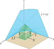
Solution Since we use the regular partition to compute \(S_{3,2}\), each subrectangle (in this case they are squares) has sides of length \[ \Delta x=\frac{2.5-1}3=\frac12,\qquad \Delta y=\frac{2-1}2=\frac12 \] and area \(\Delta A = \Delta x\,\Delta y = \frac14\). The corresponding Riemann sum is \[ S_{3,2} = \sum_{i=1}^3\sum_{j=1}^2 f(P_{ij})\,\Delta A = \frac14 \sum_{i=1}^3\sum_{j=1}^2 f(P_{ij}) \] where \(f(x,y)=xy\).
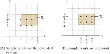
- (a) If we use the lower-left vertices shown in Figure 15.8, the Riemann sum is \[ \begin{array}{rl} S_{3,2} &= \tfrac14 \left(f(1,1)+f\big(1,\tfrac32\big)+f\big(\tfrac32,1\big)+f\big(\tfrac32,\tfrac32\big)+f(2,1)+f\big(2,\tfrac32\big)\right)\\ &= \tfrac14 \big(1 + \tfrac32 + \tfrac32 + \tfrac94 + 2+3 \big)= \tfrac14\big(\tfrac{45}4\big) = 2.8125 \end{array} \]
- (b) Using the midpoints of the rectangles shown in Figure 15.8, we obtain \[ \begin{array}{rl} S_{3,2} &= \tfrac14 \!\left( f\!\left(\tfrac54,\tfrac54\right) + f\!\left(\tfrac54,\tfrac74\right) + f\!\left(\tfrac74,\tfrac54\right) + f\!\left(\tfrac74,\tfrac74\right) + f\big(\tfrac94,\tfrac54\big) + f\big(\tfrac94,\tfrac74\big) \right)\\ &= \tfrac14 \big(\tfrac{25}{16}+\tfrac{35}{16} +\tfrac{35}{16}+\tfrac{49}{16}+\tfrac{45}{16}+\tfrac{63}{16} \big)= \tfrac14\big(\tfrac{252}{16}\big) = 3.9375 \end{array} \]
864
EXAMPLE 2
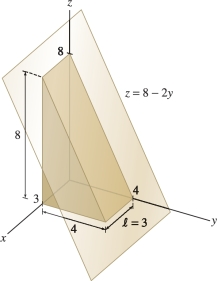
Evaluate \(\iint_{{\mathcal{R}}\,} (8-2y)\,dA\), where \({\mathcal{R}} = [0,3]\times [0,4]\).
Solution Figure 15.9 shows the graph of \(z = 8 - 2y\). The double integral is equal to the volume \(V\) of the solid wedge underneath the graph. The triangular face of the wedge has area \(A =\frac12(8)4=16\). The volume of the wedge is equal to the area \(A\) times the length \(\ell = 3\); that is, \(V=\ell A = 3(16)=48\). Therefore, \[ \iint_{{\mathcal{R}}\,} (8-2y)\,dA=48 \]
The next theorem assures us that continuous functions are integrable. Since we have not yet defined continuity at boundary points of a domain, for the purposes of the next theorem, we define continuity on \({\mathcal{R}}\) to mean that \(f\) is defined and continuous on some open set containing \({\mathcal{R}}\). We omit the proof, which is similar to the single-variable case.
THEOREM 1 Continuous Functions Are Integrable
If \(f(x,y)\) is continuous on a rectangle \({\mathcal{R}}\), then \(f(x,y)\) is integrable over \({\mathcal{R}}\).
As in the single-variable case, we often make use of the linearity properties of the double integral. They follow from the definition of the double integral as a limit of Riemann sums.
THEOREM 2 Linearity of the Double Integral
Assume that \(f(x,y)\) and \(g(x,y)\) are integrable over a rectangle \({\mathcal{R}}\). Then:
- (i) \(\iint_{{\mathcal{R}}\,} \big(f(x,y) + g(x,y)\big)\, dA = \iint_{{\mathcal{R}}\,} f(x,y) \, dA + \iint_{{\mathcal{R}}\,} g(x,y) \, dA\)
- (ii) For any constant \(C\), \(\iint_{{\mathcal{R}}\,} C f(x,y)\, dA = C\iint_{{\mathcal{R}}\,} f(x,y)\, dA\)
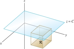
If \(f(x,y)=C\) is a constant function, then \[ \boxed{ \iint_{{\mathcal{R}}\,} C\,dA = C\cdot \mathrm{Area}({\mathcal{R}})} \]
The double integral is the signed volume of the box of base \({\mathcal{R}}\) and height \(C\) Figure 15.10. If \(C<0\), then the rectangle lies below the \(xy\)-plane, and the integral is equal to the signed volume, which is negative.
EXAMPLE 3 Arguing by Symmetry
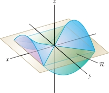
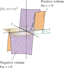
Use symmetry to show that \( \iint_{{\mathcal{R}}\,} xy^2\,dA = 0\), where \({\mathcal{R}} = [-1,1]\times [-1,1]\).
Solution The double integral is the signed volume of the region between the graph of \(f(x,y)=xy^2\) and the \(xy\)-plane Figure 15.11. However, \(f(x,y)\) takes opposite values at \((x,y)\) and \((-x,y)\): \[ f(-x,y)= -xy^2=-f(x,y) \]
Because of symmetry, the (negative) signed volume of the region below the \(xy\)-plane where \(-1\le x \le 0\) cancels with the (positive) signed volume of the region above the \(xy\)-plane where \(0\le x \le 1\). The net result is \( \iint_{{\mathcal{R}}\,} xy^2\,dA = 0\).
Iterated Integrals
865
Our main tool for evaluating double integrals is the Fundamental Theorem of Calculus (FTC), as in the single-variable case. To use the FTC, we express the double integral as an iterated integral, which is an expression of the form \[ \int_a^b\left(\int_c^d f(x,y)\,dy\right)dx \]
We often omit the parentheses in the notation for an iterated integral: \[ \int_a^b \int_c^d f(x,y)\,dy\,dx \] The order of the variables in \(dy\,dx\) tells us to integrate first with respect to \(y\) between the limits \(y=c\) and \(y=d\).
Iterated integrals are evaluated in two steps. Step One: Hold \(x\) constant and evaluate the inner integral with respect to \(y\). This gives us a function of \(x\) alone: \[ S(x) = \int_c^d f(x,y)\,dy \]
Step Two: Integrate the resulting function \(S(x)\) with respect to \(x\).
EXAMPLE 4
Evaluate \(\int_2^4 \left(\int_1^9 ye^x\,dy\right)\,dx\).
Solution First evaluate the inner integral, treating \(x\) as a constant: \[ S(x) = \int_1^9 ye^x\,dy = e^x\int_1^9 y\,dy = e^x\left(\frac12y^2\right)\bigg|_{y=1}^9 = e^x\left(\frac{81-1}2\right)=40e^x \]
Then integrate \(S(x)\) with respect to \(x\): \[ \int_2^4 \left(\int_1^9 ye^x\,dy\right) \,dx = \int_2^4 40e^x\,dx = 40e^x\bigg|_2^4= 40(e^4-e^2) \]
In an iterated integral where \(dx\) precedes \(dy\), integrate first with respect to \(x\): \[ \int_c^d\int_a^b f(x,y)\,dx\,dy = \int_{y=c}^d \left(\int_{x=a}^b f(x,y)\,dx\right)\,dy \]
Sometimes for clarity, as on the right-hand side here, we include the variables in the limits of integration.
EXAMPLE 5
Evaluate \(\int_{y=0}^4\int_{x=0}^3\frac{dx\,dy}{\sqrt{3x+4y}}\).
Solution We evaluate the inner integral first, treating \(y\) as a constant. Since we are integrating with respect to \(x\), we need an antiderivative of \(1/{\sqrt{3x+4y}}\) as a function of \(x\). We can use \(\tfrac23\sqrt{3x+4y}\) because \[ \frac{\partial }{\partial x}\left(\frac23\sqrt{3x+4y}\right) = \frac1{\sqrt{3x+4y}} \]
Thus we have \[ \begin{array}{rl} \int_{x=0}^3\frac{dx}{\sqrt{3x+4y}} &=\frac23\sqrt{3x+4y}\bigg|_{x=0}^{3} = \frac23\left(\sqrt{4y+9}-\sqrt{4y}\right)\\ \int_{y=0}^4\int_{x=0}^3\frac{dx\,dy}{\sqrt{3x+4y}} &=\frac23\int_{y=0}^4\left(\sqrt{4y+9}-\sqrt{4y}\right)\,dy \end{array} \]
866
Therefore, we have: \[ \begin{array}{rl} \int_{y=0}^4\int_{x=0}^3\frac{dx\,dy}{\sqrt{3x+4y}}&= \frac23\left(\frac16(4y+9)^{3/2}-\frac16(4y)^{3/2}\right)\bigg|_{y=0}^{4}\\ &= \frac19\left(25^{3/2}-16^{3/2} -9^{3/2} \right) = \frac{34}9 \end{array} \]
EXAMPLE 6 Reversing the Order of Integration
Verify that \[ \int_{y=0}^4\int_{x=0}^3\frac{dx\,dy}{\sqrt{3x+4y}}=\int_{x=0}^3\int_{y=0}^4\frac{dy\,dx}{\sqrt{3x+4y}} \]
Solution We evaluated the iterated integral on the left in the previous example. We compute the integral on the right and verify that the result is also \(\frac{34}9\): \[ \begin{array}{rcl} \int_{y=0}^4\frac{dy}{\sqrt{3x+4y}} &=&\frac12\sqrt{3x+4y}\bigg|_{y=0}^{4} = \frac12(\sqrt{3x+16}-\sqrt{3x})\\ \int_{x=0}^3\int_{y=0}^4\frac{dy\,dx}{\sqrt{3x+4y}} &=&\frac12\int_0^3(\sqrt{3x+16}-\sqrt{3x})\,dy \\ &=& \frac12\Big(\frac29(3x+16)^{3/2}-\frac29(3x)^{3/2}\Big)\bigg|_{x=0}^{3} \\ &=& \frac19\left(25^{3/2}-9^{3/2} -16^{3/2}\right) = \frac{34}9 \end{array} \]
The previous example illustrates a general fact: The value of an iterated integral does not depend on the order in which the integration is performed. This is part of Fubini’s Theorem. Even more important, Fubini’s Theorem states that a double integral over a rectangle can be evaluated as an iterated integral.
CAUTION
When you reverse the order of integration in an iterated integral, remember to interchange the limits of integration (the inner limits become the outer limits).
THEOREM 3 Fubini’s Theorem
The double integral of a continuous function \(f(x,y)\) over a rectangle \({\mathcal{R}}=[a,b]\times[c,d]\) is equal to the iterated integral (in either order): \[ \iint_{{\mathcal{R}}\,} f(x,y)\,dA = \int_{x=a}^b\int_{y=c}^d f(x,y)\,dy\,dx = \int_{y=c}^d\int_{x=a}^b f(x,y)\,dx\,dy \]
Proof We sketch the proof. We can compute the double integral as a limit of Riemann sums that use a regular partition of \({\mathcal{R}}\) and sample points \(P_{ij} = (x_i,y_j)\), where \(\{x_i\}\) are sample points for a regular partition on \([a,b]\), and \(\{y_j\}\) are sample points for a regular partition of \([c,d]\): \[ \iint_{{\mathcal{R}}\,} f(x,y)\,dA = \lim_{N,M \to \infty} \sum^N_{i=1} \sum^M_{j=1} f(x_i, y_j) \Delta y \Delta x \]
Here \(\Delta x = (b-a)/N\) and \(\Delta y = (d-c)/M\). Fubini’s Theorem stems from the elementary fact that we can add up the values in the sum in any order. So if we list the values \(f(P_{ij})\) in an \(N \times M\) array as shown in the margin, we can add up the columns first and then add up the column sums. This yields \[ \iint_{{\mathcal{R}}\,} f(x,y)\,dA = \lim_{N,M \to \infty} \sum^N_{i=1} \underbrace{\left( \sum^M_{j=1} f(x_i, y_j) \Delta y \right)}_{\mbox{First sum the columns;}\atop \mbox{ then add up the column sums.}} \Delta x \]
| \(3\) | \(f(P_{13})\) | \(f(P_{23})\) | \(f(P_{33})\) |
| \(2\) | \(f(P_{12})\) | \(f(P_{22})\) | \(f(P_{32})\) |
| \(1\) | \(f(P_{11})\) | \(f(P_{21})\) | \(f(P_{31})\) |
| \(j\) / \(i\) | \(1\) | \(2\) | \(3\) |
867
For fixed \(i\), \(f(x_i,y)\) is a continuous function of \(y\) and the inner sum on the right is a Riemann sum that approaches the single integral \(\int_c^d f(x_i,y)\,dy\). In other words, setting \(S(x)=\int_c^df(x,y)\,dy\), we have \[ \lim_{M\to\infty}\sum_{j=1}^M f(x_i,y_j)=\int_c^d f(x_i,y)\,dy = S(x_i) \]
To complete the proof, we take two facts for granted. First, that \(S(x)\) is a continuous function for \(a\le x\le b\). Second, that the limit as \(N\), \(M\to\infty\) may be computed by taking the limit first with respect to \(M\) and then with respect to \(N\). Granting this, \[ \begin{array}{rl} \iint_{{\mathcal{R}}\,} f(x,y)\,dA &= \lim_{N \to \infty}\sum_{i=1}^N\left( \lim_{M \to \infty}\sum^M_{j=1} f(x_i, y_j) \Delta y \right) \Delta x =\lim_{N\to\infty}\sum_{i=1}^N S(x_i) \Delta x \\ &= \int_a^b S(x)\,dx=\int_a^b\left(\int_c^df(x,y)\,dy\right)\,dx \end{array} \]
Note that the sums on the right in the first line are Riemann sums for \(S(x)\) that converge to the integral of \(S(x)\) in the second line. This proves Fubini’s Theorem for the order \(dy\,dx\). A similar argument applies to the order \(dx\,dy\).
GRAPHICAL INSIGHT
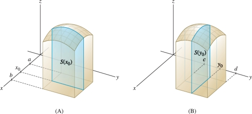
When we write a double integral as an iterated integral in the order \(dy\,dx\), then for each fixed value \(x=x_0\), the inner integral is the area of the cross section of \(S\) in the vertical plane \(x=x_0\) perpendicular to the \(x\)-axis (Figure 15.12): \[ S(x_0) = \int_c^d f(x_0,y)\,dy = \begin{array}{l} \mbox{area of cross section in vertical plane}\\ x=x_0\mbox{ perpendicular to the }x\mbox{-axis} \end{array} \]
What Fubini’s Theorem says is that the volume \(V\) of \(S\) can be calculated as the integral of cross-sectional area \(S(x)\): \[ V = \int_a^b\int_c^d f(x,y)\,dy\,dx = \int_a^b S(x)\,dx = \textrm{integral of cross-sectional area} \]
Similarly, the iterated integral in the order \(dx\,dy\) calculates \(V\) as the integral of cross sections perpendicular to the \(y\)-axis (Figure 15.12).
868
EXAMPLE 7
Find the volume \(V\) between the graph of \(f(x,y) = 16-x^2-3y^2\) and the rectangle \({\mathcal{R}}=[0,3]\times[0,1]\) Figure 15.13.
Solution The volume \(V\) is equal to the double integral of \(f(x,y)\), which we write as an iterated integral: \[ V=\iint_{{\mathcal{R}}\,}(16-x^2-3y^2)\,dA =\int_{x=0}^3\int_{y=0}^1(16-x^2-3y^2)\,dy\,dx \]
We evaluate the inner integral first and then compute \(V\): \[ \begin{array}{rl} &\int_{y=0}^1(16-x^2-3y^2)\,dy = (16y-x^2y- y^3)\bigg|_{y=0}^1 =15 -x^2\\ &V = \int_{x=0}^3 (15 -x^2)\,dx = \left(15x-\frac13x^3 \right)\bigg|_0^3 = 36 \end{array} \]
EXAMPLE 8
Calculate \(\iint_{{\mathcal{R}}\,} \frac{dA}{(x+y)^2}\), where \({\mathcal{R}}=[1,2] \times [0,1]\) Figure 15.14.

Solution \[ \begin{array}{rl} \iint_{{\mathcal{R}}\,} \frac{dA}{(x+y)^2} &= \int_{x=1}^2\left(\int_{y=0}^1 \frac{dy}{(x+y)^2}\right) dx = \int_1^2\left(-\frac1{x+y}\bigg|_{y=0}^1 \right)\,dx\\ &= \int_1^2\left(-\frac1{x+1} + \frac1{x} \right) dx = \bigl(\ln x - \ln(x+1)\bigr)\bigg|_1^2 \\ & = \bigl(\ln 2 - \ln 3\bigr)-\bigl(\ln 1-\ln 2\bigr) = 2\ln 2-\ln 3 = \ln \frac43 \end{array} \]
When the function is a product \(f(x,y)=g(x)h(y)\), the double integral over a rectangle is simply the product of the single integrals. We verify this by writing the double integral as an iterated integral. If \({\mathcal{R}} = [a,b]\times [c,d]\), \begin{equation} \begin{array}{rcl} \iint_{{\mathcal{R}}\,} g(x)h(y)\,dA &=& \int_a^b \left(\int_c^d g(x)h(y)\,dy\right)dx = \int_a^b g(x)\left(\int_c^d h(y)\,dy\right)dx\\ &=& \left(\int_a^b g(x)\,dx\right)\left(\int_c^d h(y)\,dy\right) \end{array} \end{equation}
EXAMPLE 9 Iterated Integral of a Product Function
Calculate \[ \int_0^{2}\int_0^{\pi/2}e^x\cos y\,dy\,dx \]
Solution The integrand \(f(x,y) = e^x \cos y\) is a product, so we obtain \[ \begin{array}{rl} \int_0^{2}\int_0^{\pi/2}e^x\cos y\, dy\,dx &=\left(\int_0^{2}e^x \, dx\right) \left(\int_0^{\pi/2}\cos y\, dy\right) = \left( e^x\bigg|_0^2\right) \left( \sin y \bigg|_0^{\pi/2}\right)\\ & = (e^2-1)(1)=e^2-1 \end{array} \]
15.1.1 Summary
869
- A Riemann sum for \(f(x,y)\) on a rectangle \({\mathcal{R}}=[a,b] \times [c,d]\) is a sum of the form \[ S_{N,M} = \sum_{i=1}^N\sum_{j=1}^M f(P_{ij})\,\Delta x_i\,\Delta y_j \] corresponding to partitions of \([a,b]\) and \([c,d]\), and choice of sample points \(P_{ij}\) in the subrectangle \({\mathcal{R}}_{ij}\).
- The double integral of \(f(x,y)\) over \({\mathcal{R}}\) is defined as the limit (if it exists): \[ \iint_{{\mathcal{R}}\,} f(x,y)\,dA = \lim_{M,N\to \infty} \sum_{i=1}^N\sum_{j=1}^M f(P_{ij})\,\Delta x_i\,\Delta y_j \] We say that \(f(x,y)\) is integrable over \({\mathcal{R}}\) if this limit exists.
- A continuous function on a rectangle \({\mathcal{R}}\) is integrable.
- The double integral is equal to the signed volume of the region between the graph of \(z=f(x,y)\) and the rectangle \({\mathcal{R}}\). The signed volume of a region is positive if it lies above the \(xy\)-plane and negative if it lies below the \(xy\)-plane.
- If \(f(x,y)=C\) is a constant function, then \[ \iint_{{\mathcal{R}}\,} C\,dA = C\cdot \textrm{Area}({\mathcal{R}}) \]
- Fubini’s Theorem: The double integral of a continuous function \(f(x,y)\) over a rectangle \({\mathcal{R}} = [a,b]\times [c,d]\) can be evaluated as an iterated integral (in either order): \[ \iint_{{\mathcal{R}}\,} f(x,y)\,dA = \int_{x=a}^b \int_{y=c}^d f(x,y)\,dy\, dx = \int_{y=c}^d \int_{x=a}^b f(x,y)\,dx\,dy \]