15.2 Double Integrals over More General Regions
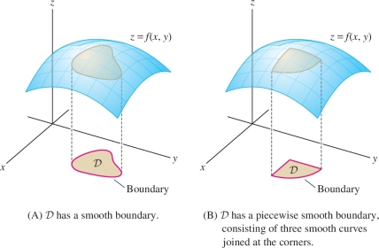
In the previous section, we restricted our attention to rectangular domains. Now we shall treat the more general case of domains \({\mathcal{D}}\) whose boundaries are simple closed curves (a curve is simple if it does not intersect itself). We assume that the boundary of \({\mathcal{D}}\) is smooth as in Figure 15.15 or consists of finitely many smooth curves, joined together with possible corners, as in Figure 15.15. A boundary curve of this type is called piecewise smooth. We also assume that \({\mathcal{D}}\) is a closed domain; that is, \({\mathcal{D}}\) contains its boundary.
Fortunately, we do not need to start from the beginning to define the double integral over a domain \({\mathcal{D}}\) of this type. Given a function \(f(x,y)\) on \({\mathcal{D}}\), we choose a rectangle \({\mathcal{R}} = [a,b]\times[c,d]\) containing \({\mathcal{D}}\) and define a new function \(\tilde f (x,y)\) that agrees with \(f(x,y)\) on \({\mathcal{D}}\) and is zero outside of \({\mathcal{D}}\) Figure 15.16: \[ \tilde{f}(x,y) = \begin{cases} f(x,y) & \textrm{if }(x,y)\in{\mathcal{D}} \\ 0 & \textrm{if }(x,y)\notin{\mathcal{D}} \end{cases} \]
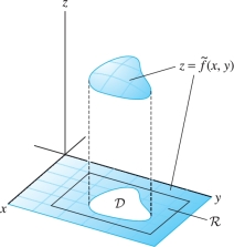
The double integral of \(f\) over \({\mathcal{D}}\) is defined as the integral of \(\tilde{f}\) over \({\mathcal{R}}\): \begin{equation*} \boxed{ \iint_{{\mathcal{D}}\,} f(x,y)\,dA = \iint_{{\mathcal{R}}\,} \tilde{f}(x,y)\,dA}\tag{1} \end{equation*}
We say that \(f\) is integrable over \({\mathcal{D}}\) if the integral of \(\tilde{f}\) over \({\mathcal{R}}\) exists. The value of the integral does not depend on the particular choice of \({\mathcal{R}}\) because \(\tilde{f}\) is zero outside of \({\mathcal{D}}\).
873
This definition seems reasonable because the integral of \(\tilde{f}\) only “picks up” the values of \(f\) on \({\mathcal{D}}\). However, \(\tilde{f}\) is likely to be discontinuous because its values jump suddenly to zero beyond the boundary. Despite this possible discontinuity, the next theorem guarantees that the integral of \(\tilde{f}\) over \({\mathcal{R}}\) exists if our original function \(f\) is continuous.
THEOREM 1
If \(f(x,y)\) is continuous on a closed domain \({\mathcal{D}}\) whose boundary is a closed, simple, piecewise smooth curve, then \(\iint_{{\mathcal{D}}\,} f(x,y)\,dA\) exists.
In Theorem 1, we define continuity on \({\mathcal{D}}\) to mean that \(f\) is defined and continuous on some open set containing \({\mathcal{D}}\).
As in the previous section, the double integral defines the signed volume between the graph of \(f(x,y)\) and the \(xy\)-plane, where regions below the \(xy\)-plane are assigned negative volume.
We can approximate the double integral by Riemann sums for the function \(\tilde{f}\) on a rectangle \({\mathcal{R}}\) containing \({\mathcal{D}}\). Because \(\tilde{f}(P) = 0\) for points \(P\) in \({\mathcal{R}}\) that do not belong to \({\mathcal{D}}\), any such Riemann sum reduces to a sum over those sample points that lie in \({\mathcal{D}}\): \begin{equation*} \iint_{{\mathcal{D}}\,} f(x,y)\,dA \approx \sum_{i=1}^N\sum_{j=1}^M \tilde{f}(P_{ij})\,\Delta x_i\,\Delta y_j = \underbrace{\sum f(P_{ij})\,\Delta x_i\,\Delta y_j}_{\mbox{Sum only over points} \atop {P_{ij}\mbox{ that lie in }{\mathcal{D}}}}\tag{2} \end{equation*}
EXAMPLE 1
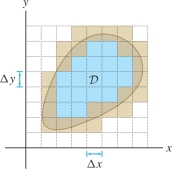
Compute \(S_{4,4}\) for the integral \(\iint_{{\mathcal{D}}\,} (x+y)\,dA\), where \({\mathcal{D}}\) is the shaded domain in Figure 15.17. Use the upper right-hand corners of the squares as sample points.
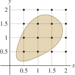
Solution Let \(f(x,y) = x+y\). The subrectangles in Figure 15.17 have sides of length \(\Delta x = \Delta y = \frac12\) and area \(\Delta A = \frac14\). Only \(7\) of the 16 sample points lie in \({\mathcal{D}}\), so \[ \begin{array}{rcl} S_{4,4} &=& \sum_{i=1}^4\sum_{j=1}^4 \tilde{f}(P_{ij})\,\Delta x\,\Delta y=\frac14\big(f(0.5,0.5)+f(1,0.5) +f(0.5,1)+f(1,1)\\ &&+f(1.5,1)+f(1,1.5)+f(1.5,1.5)\big)\\ &=&\frac14\bigl(1+1.5 +1.5+2 +2.5 +2.5+3\bigr) =\frac72 \end{array} \]
The linearity properties of the double integral carry over to general domains: If \(f(x,y)\) and \(g(x,y)\) are integrable and \(C\) is a constant, then \[ \begin{array}{rl} \iint_{{\mathcal{D}}\,} (f(x,y)+g(x,y))\,dA &=\iint_{{\mathcal{D}}\,} f(x,y) \,dA + \iint_{{\mathcal{D}}\,} g(x,y) \,dA\\ \iint_{{\mathcal{D}}\,} Cf(x,y) \,dA &= C\iint_{{\mathcal{D}}\,} f(x,y) \,dA \end{array} \]
Although we usually think of double integrals as representing volumes, it is worth noting that we can express the area of a domain \({\mathcal{D}}\) in the plane as the double integral of the constant function \(f(x,y)=1\): \begin{equation*} \boxed{\textrm{Area}({\mathcal{D}}) = \iint_{{\mathcal{D}}\,} 1\,dA}\tag{3} \end{equation*}
874
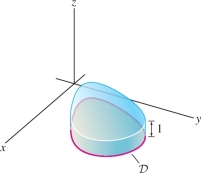
Indeed, as we see in Figure 15.18, the the area of \({\mathcal{D}}\) is equal to the volume of the “cylinder” of height \(1\) with \({\mathcal{D}}\) as base. More generally, for any constant \(C\), \begin{equation*} \iint_{{\mathcal{D}}\,} C\,dA = C \,\textrm{Area}({\mathcal{D}})\tag{4} \end{equation*}
CONCEPTUAL INSIGHT
Eq. (3) tells us that we can approximate the area of a domain \({\mathcal{D}}\) by a Riemann sum for \(\iint_{{\mathcal{D}}\,} 1\,dA\). In this case, \(f(x,y)=1\), and we obtain a Riemann sum by adding up the areas \(\Delta x_i\,\Delta y_j\) of those rectangles in a grid that are contained in \({\mathcal{D}}\) or that intersects the boundary of \({\mathcal{D}}\) Figure 15.19. The finer the grid, the better the approximation. The exact area is the limit as the sides of the rectangles tend to zero.
Regions between Two Graphs
When \({\mathcal{D}}\) is a region between two graphs in the \(xy\)-plane, we can evaluate double integrals over \({\mathcal{D}}\) as iterated integrals. We say that \({\mathcal{D}}\) is vertically simple if it is the region between the graphs of two continuous functions \(y={g_1}(x)\) and \(y = g_2(x)\) (Figure 15.20): \[ {\mathcal{D}} = \{(x,y): a\le x \le b,\quad {g_1}(x) \le y \le g_2(x)\} \]
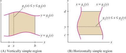
Similarly, \({\mathcal{D}}\) is horizontally simple if \[ {\mathcal{D}} = \{(x,y): c\le y \le d,\quad {g_1}(y) \le x \le g_2(y)\} \]
When you write a double integral over a vertically simple region as an iterated integral, the inner integral is an integral over the dashed segment shown in Figure 15.20. For a horizontally simple region, the inner integral is an integral over the dashed segment shown in Figure 15.20.
THEOREM 2
If \({\mathcal{D}}\) is vertically simple with description \[ a\le x \le b,\qquad {g_1}(x) \le y \le g_2(x) \] then \[ \boxed{\iint_{{\mathcal{D}}\,} f(x,y)\, dA = \int_a^b\int_{{g_1}(x)}^{g_2(x)} f(x,y)\,dy\,dx} \]
If \({\mathcal{D}}\) is a horizontally simple region with description \[ c\le y \le d,\qquad {g_1}(y) \le x \le g_2(y) \] then \[ \boxed{\iint_{{\mathcal{D}}\,} f(x,y)\, dA = \int_c^d\int_{{g_1}(y)}^{g_2(y)} f(x,y)\,dx\,dy} \]
875
Proof We sketch the proof, assuming that \({\mathcal{D}}\) is vertically simple (the horizontally simple case is similar). Choose a rectangle \({\mathcal{R}} = [a,b]\times[c,d]\) containing \({\mathcal{D}}\). Then \begin{equation*} \iint_{{\mathcal{D}}\,} f(x,y)\, dA = \int_a^b \int_c^d \tilde f(x,y)\,dy\,dx\tag{5} \end{equation*}
Although \(\tilde f\) need not be continuous, the use of Fubini’s Theorem in Eq. (5) can be justified. In particular, the integral \(\int_c^d \tilde f(x,y)\,dy\) exists and is a continuous function of \(x\).
By definition, \(\tilde f(x,y)\) is zero outside \({\mathcal{D}}\), so for fixed \(x\), \(\tilde f(x,y)\) is zero unless \(y\) satisfies \({g_1}(x)\le y \le g_2(x)\). Therefore, \[ \int_c^d \tilde f(x,y)\,dy = \int_{{g_1}(x)}^{g_2(x)} f(x,y)\,dy \]
Substituting in Eq. (5), we obtain the desired equality: \[ \iint_{{\mathcal{D}}\,} f(x,y)\, dA = \int_a^b\int_{{g_1}(x)}^{g_2(x)} f(x,y)\,dy\,dx \]
Integration over a simple region is similar to integration over a rectangle with one difference: The limits of the inner integral may be functions instead of constants.
EXAMPLE 2
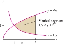
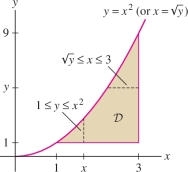
Evaluate \(\iint_{{\mathcal{D}}\,}x^2y\,dA\), where \({\mathcal{D}}\) is the region in Figure 15.21.
Solution
Step 1. Describe \({\mathcal{D}}\) as a vertically simple region.
\[ \underbrace{\,\,1\le x \le 3\,\,}_{\mbox{ Limits of outer}\atop \mbox{ integral}},\quad\qquad \underbrace{\,\,\frac1x\le y \le \sqrt{x}\,\,}_{\mbox{Limits of inner}\atop \mbox{ integral}} \] In this case, \(g_1(x)=1/x\) and \(g_2(x)=\sqrt{x}\).
Step 2. Set up the iterated integral.
\[ \iint_{{\mathcal{D}}\,} x^2y\,dA = \int_1^3\int_{y=1/x}^{\sqrt{x}} x^2y\,dy\,dx \] Notice that the inner integral is an integral over a vertical segment between the graphs of \(y={1}/{x}\) and \(y=\sqrt{x}\).
Step 3. Compute the iterated integral.
As usual, we evaluate the inner integral by treating \(x\) as a constant, but now the upper and lower limits depend on \(x\): \[ \int_{y=1/x}^{\sqrt{x}}x^2y\,dy = \frac12x^2y^2 \bigg|_{y=1/x}^{\sqrt{x}} =\frac12x^2(\sqrt{x})^2 - \frac12x^2\left(\frac1{x}\right)^2 = \frac12x^3-\frac12 \]
We complete the calculation by integrating with respect to \(x\): \[ \begin{array}{rl} \iint_{{\mathcal{D}}\,} x^2y\,dA = \int_1^3\left(\frac12x^3-\frac12\right) \,dx = \left(\frac18x^4-\frac12x\right)\bigg|_1^3 \\ &= \frac{69}8 - \left(-\frac38\right)=9 \end{array} \]
876
EXAMPLE 3 Horizontally Simple Description Better
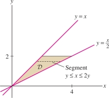
Find the volume \(V\) of the region between the plane \(z=2x+3y\) and the triangle \({\mathcal{D}}\) in Figure 15.22.
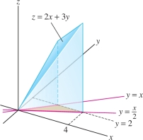
Solution The triangle \({\mathcal{D}}\) is bounded by the lines \(y=x/2\), \(y=x\), and \(y=2\). We see in Figure 15.23 that \({\mathcal{D}}\) is vertically simple, but the upper curve is not given by a single formula: The formula switches from \(y=x\) to \(y=2\). Therefore, it is more convenient to describe \({\mathcal{D}}\) as a horizontally simple region Figure 15.23: \[ {\mathcal{D}}: 0\le y \le 2,\quad y \le x \le 2y \]
The volume is equal to the double integral of \(f(x,y)=2x+3y\) over \({\mathcal{D}}\), \[ \begin{array}{rl} V &=\iint_{{\mathcal{D}}\,} f(x,y)\,dA = \int_0^2\int_{x=y}^{2y} (2x+3y)\,dx\,dy \\ &=\int_0^2\big( x^2+3yx\big)\bigg|_{x=y}^{2y}\,dy = \int_0^2\big( (4y^2+6y^2) - (y^2+3y^2) \big)\,dy\\ & =\int_0^2 6y^2 \, dy = 2y^3\bigg|_0^2=16 \end{array} \]
The next example shows that in some cases, one iterated integral is easier to evaluate than the other.
EXAMPLE 4 Choosing the Best Iterated Integral
Evaluate \(\iint_{{\mathcal{D}}\,} e^{y^2}dA\) for \({\mathcal{D}}\) in Figure 15.24.
877
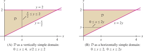
Solution First, let’s try describing \({\mathcal{D}}\) as a vertically simple domain. Referring to Figure 15.24, we have \[ {\mathcal{D}}: 0\le x \le 4,\quad \dfrac12 x \leq y \leq 2 \quad\Rightarrow\quad \iint_{{\mathcal{D}}\,} e^{y^2}\,dA=\int_{x=0}^4 \int_{y=x/2}^2 e^{y^2}\,dy\,dx \]
The inner integral cannot be evaluated because we have no explicit antiderivative for \(e^{y^2}\). Therefore, we try describing \({\mathcal{D}}\) as horizontally simple [Figure 15.24]: \[ {\mathcal{D}}: 0\le y \le 2,\quad 0 \le x \le 2y \]
This leads to an iterated integral that can be evaluated: \[ \begin{array}{rcl} \int_{0}^2 \int_{x=0}^{2y} e^{y^2}\,dx\,dy &=& \int_{0}^2 \Big( xe^{y^2}\Big|_{x=0}^{2y}\Big) \,dy = \int_{0}^2 2ye^{y^2} \,dy\\ &=& e^{y^2}\Big|_0^2 = e^4-1 \end{array} \]
EXAMPLE 5 Changing the Order of Integration
Sketch the domain of integration \({\mathcal{D}}\) corresponding to \[ \int_1^9\int_{\sqrt y}^3 xe^y\,dx\,dy \]
Then change the order of integration and evaluate.
Solution The limits of integration give us inequalities that describe the domain \({\mathcal{D}}\) (as a horizontally simple region since \(dx\) precedes \(dy\)): \[ 1\le y \le 9,\qquad \sqrt{y} \le x \le 3 \]
We sketch the region in Figure 15.25. Now observe that \({\mathcal{D}}\) is also vertically simple: \[ 1\le x \le 3,\qquad 1 \le y \le x^2 \] so we can rewrite our integral and evaluate: \[ \begin{array}{rl} \int_1^9\int_{x=\sqrt y}^3 xe^y\,dx\,dy&=\int_1^3 \int_{y=1}^{x^2} xe^{y}\,dy\,dx =\int_1^3\left( \int_{y=1}^{x^2} xe^{y}\,dy \right)\,dx\\ &= \int_1^3 \Big(xe^y\Big|_{y=1}^{x^2}\Big)\,dx =\int_1^3 (xe^{x^2}-ex)\,dx = \frac12(e^{x^2}-ex^2)\Big|_1^3\\ & = \frac12(e^9-9e)-0 = \frac12 (e^9 - 9e) \end{array} \]
878
In the next theorem, part (a) is a formal statement of the fact that larger functions have larger integrals, a fact that we also noted in the single-variable case. Part (b) is useful for estimating integrals.
THEOREM 3
Let \(f(x,y)\) and \(g(x,y)\) be integrable functions on \({\mathcal{D}}\).
- (a) If \(f(x,y)\le g(x,y)\) for all \((x,y)\in {\mathcal{D}}\), then \begin{equation*} \iint_{{\mathcal{D}}\,} f(x,y)\,dA \le \iint_{{\mathcal{D}}\,} g(x,y)\,dA\tag{6} \end{equation*}
- (b) If \(m\le f(x,y)\le M\) for all \((x,y) \in {\mathcal{D}}\), then \begin{equation*} m\,\textrm{Area}({\mathcal{D}}) \le \iint_{{\mathcal{D}}\,} f(x,y)\,dA \le M\,\textrm{Area}({\mathcal{D}})\tag{7} \end{equation*}
Proof If \(f(x,y)\le g(x,y)\), then every Riemann sum for \(f(x,y)\) is less than or equal to the corresponding Riemann sum for \(g\): \[ \sum f(P_{ij})\,\Delta x_i\,\Delta y_j \le \sum g(P_{ij})\,\Delta x_i\,\Delta y_j \]
We obtain (6) by taking the limit. Now suppose that \(f(x,y)\le M\) and apply (6) with \(g(x,y)=M\): \[ \iint_{{\mathcal{D}}\,} f(x,y)\,dA \le \iint_{{\mathcal{D}}\,} M\,dA = M\,\textrm{Area}({\mathcal{D}}) \]
This proves half of (7). The other half follows similarly.
EXAMPLE 6
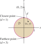
Estimate \(\iint_{\mathcal{D}}\,\frac{dA}{\sqrt{x^2+(y-2)^2}}\) where \({\mathcal{D}}\) is the disk of radius 1 centered at the origin.
Solution The quantity \(\sqrt{x^2+(y-2)^2}\) is the distance \(d\) from \((x,y)\) to \((0,2)\), and we see from Figure 15.26 that \(1\le d\le 3\). Taking reciprocals, we have \[ \frac13\le \frac1{\sqrt{x^2+(y-2)^2}}\le 1 \]
We apply (7) with \(m=\frac13\) and \(M=1\), using the fact that \(\textrm{Area}({\mathcal{D}})=\pi\), to obtain \[ \frac{\pi}3 \le \iint_{{\mathcal{D}}}\,\frac{dA}{\sqrt{x^2+(y-2)^2}}\le \pi \]
REMINDER
Equation (8) is similar to the definition of an average value in one variable: \[ \overline{f} = \frac1{b-a}\int_a^b\,f(x)\,dx = \frac{\int_a^b\,f(x)\,dx}{\int_a^b\,1\,dx} \]
The average value (or mean value) of a function \(f(x,y)\) on a domain \({\mathcal{D}}\), which we denote by \(\overline{f}\), is the quantity \begin{equation*} \boxed{\overline{f} = \frac1{\textrm{Area}({\mathcal{D}})}\iint_{{\mathcal{D}}\,} f(x,y)\,dA = \frac{\iint_{{\mathcal{D}}\,} f(x,y)\,dA}{\iint_{{\mathcal{D}}\,} 1\,dA}}\tag{8} \end{equation*}
879
Equivalently, \(\overline{f}\) is the value satisfying the relation \[ \boxed{\iint_{{\mathcal{D}}\,} f(x,y)\,dA = \overline{f}\cdot\textrm{Area}({\mathcal{D}})} \]
GRAPHICAL INSIGHT
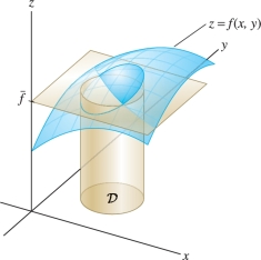
The solid region under the graph has the same (signed) volume as the cylinder with base \({\mathcal{D}}\) of height \(\overline{f}\) Figure 15.27.
EXAMPLE 7
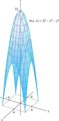
An architect needs to know the average height \(\overline{H}\) of the ceiling of a pagoda whose base \({\mathcal{D}}\) is the square \([-4,4]\times [-4,4]\) and roof is the graph of \[ H(x,y)=32-x^2-y^2 \] where distances are in feet Figure 15.28. Calculate \(\overline{H}\).
Solution First, we compute the integral of \(H(x,y)\) over \({\mathcal{D}}\): \[ \begin{array}{rl} \!\!\iint_{{\mathcal{D}}\,}(32-x^2-y^2)\,dA &=\int_{-4}^4\int_{-4}^4(32-x^2-y^2)\,dy\,dx \\ &= \int_{-4}^4 \left(\left(32y-x^2y-\frac13y^3\right)\bigg|_{-4}^4\right) dx = \int_{-4}^4 \left(\frac{640}3-8x^2\right) dx\\ &=\left(\frac{640}3x-\frac83x^3\right)\bigg|_{-4}^4 = \frac{4096}3 \end{array} \]
The area of \({\mathcal{D}}\) is \(8\times 8=64\), so the average height of the pagoda’s ceiling is \[ \overline{H} = \frac1{\textrm{Area}({\mathcal{D}})}\iint_{{\mathcal{D}}\,} H(x,y)\,dA = \frac1{64}\left(\frac{4096}3\right)=\frac{64}3\approx 21.3~\textrm{ft} \]
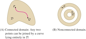
The Mean Value Theorem states that a continuous function on a domain \({\mathcal{D}}\) must take on its average value at some point \(P\) in \({\mathcal{D}}\), provided that \({\mathcal{D}}\) is closed, bounded, and also connected (see Exercise 63 for a proof). By definition, \({\mathcal{D}}\) is connected if any two points in \({\mathcal{D}}\) can be joined by a curve in \({\mathcal{D}}\) Figure 15.29.
THEOREM 4 Mean Value Theorem for Double Integrals
If \(f(x,y)\) is continuous and \({\mathcal{D}}\) is closed, bounded, and connected, then there exists a point \(P\in{\mathcal{D}}\) such that \begin{equation*} \iint_{{\mathcal{D}}\,} f(x,y)\,dA = f(P)\,\textrm{Area}({\mathcal{D}})\tag{9} \end{equation*}
Equivalently, \(f(P)=\overline{f}\), where \(\overline{f}\) is the average value of \(f\) on \({\mathcal{D}}\).
Decomposing the Domain into Smaller Domains
880
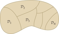
Double integrals are additive with respect to the domain: If \({\mathcal{D}}\) is the union of domains \({\mathcal{D}}_1, {\mathcal{D}}_2,\dots,{\mathcal{D}}_N\) that do not overlap except possibly on boundary curves Figure 15.30, then \[ \boxed{\iint_{{\mathcal{D}}\,} f(x,y)\, dA = \iint_{{\mathcal{D}}_1\,} f(x,y)\, dA + \cdots + \iint_{{\mathcal{D}}_N\,} f(x,y)\, dA} \]
Additivity may be used to evaluate double integrals over domains \({\mathcal{D}}\) that are not simple but can be decomposed into finitely many simple domains.
In general, the approximation (10) is useful only if \({\mathcal{D}}\) is small in both width and length, that is, if \({\mathcal{D}}\) is contained in a circle of small radius. If \({\mathcal{D}}\) has small area but is very long and thin, then \(f\) may be far from constant on \({\mathcal{D}}\).
We close this section with a simple but useful remark. If \(f(x,y)\) is a continuous function on a small domain \({\mathcal{D}}\), then \begin{equation*} \iint_{{\mathcal{D}}\,} f(x,y)\,dA \approx \underbrace{f(P)\,\textrm{Area}({\mathcal{D}})}_{\textrm{Function value }\times\textrm{ area}}\tag{10} \end{equation*} where \(P\) is any sample point in \({\mathcal{D}}\). In fact, we can choose \(P\) so that (10) is an equality by Theorem 4. But if \({\mathcal{D}}\) is small, then \(f\) is nearly constant on \({\mathcal{D}}\), and (10) holds as a good approximation for all \(P \in {\mathcal{D}}\).
If the domain \({\mathcal{D}}\) is not small, we may partition it into \(N\) smaller subdomains \({\mathcal{D}}_1, \dots, {\mathcal{D}}_N\) and choose sample points \(P_j\) in \({\mathcal{D}}_j\). By additivity, \[ \iint_{{\mathcal{D}}\,} f(x,y)\,dA = \sum_{j=1}^N \iint_{{\mathcal{D}}_j\,} f(x,y)\,dA \approx \sum_{j=1}^N f(P_j)\,\textrm{Area}({\mathcal{D}}_j) \] and thus we have the approximation \begin{equation*} \boxed{\iint_{{\mathcal{D}}\,} f(x,y)\,dA \approx \sum_{j=1}^N f(P_j)\,\textrm{Area}({\mathcal{D}}_j)}\tag{11} \end{equation*}
We can think of Eq. (11) as a generalization of the Riemann sum approximation. In a Riemann sum, \({\mathcal{D}}\) is partitioned by rectangles \({\mathcal{R}}_{ij}\) of area \(\Delta A_{ij} = \Delta x_i\,\Delta y_j\).
EXAMPLE 8
Estimate \(\iint_{{\mathcal{D}}\,} f(x,y)\,dA\) for the domain \({\mathcal{D}}\) in Figure 15.31, using the areas and function values given there and the accompanying table.
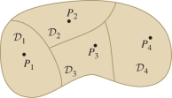
| \(j\) | \(1\) | \(2\) | \(3\) | \(4\) |
| \(\textrm{Area}({\mathcal{D}}_j)\) | \(1\) | \(1\) | \(0.9\) | \(1.2\) |
| \(f(P_j)\) | \(1.8\) | \(2.2\) | \(2.1\) | \(2.4\) |
Solution \[ \begin{array}{rl} \iint_{{\mathcal{D}}\,} f(x,y)\,dA &\approx \sum_{j=1}^4 f(P_j)\,\textrm{Area}({\mathcal{D}}_j) \\ &= (1.8)(1)+(2.2)(1) +(2.1)(0.9)+(2.4)(1.2) \approx 8.8 \end{array} \]
15.2.1 Summary
- We assume that \({\mathcal{D}}\) is a closed, bounded domain whose boundary is a simple closed curve that either is smooth or has a finite number of corners. The double integral is defined by \[ \iint_{{\mathcal{D}}\,} f(x,y)\,dA = \iint_{{\mathcal{R}}\,} \tilde{f}(x,y)\,dA \] where \({\mathcal{R}}\) is a rectangle containing \({\mathcal{D}}\) and \(\tilde{f}(x,y)=f(x,y)\) if \((x,y)\in{\mathcal{D}}\), and \(\tilde{f}(x,y)=0\) otherwise. The value of the integral does not depend on the choice of \({\mathcal{R}}\).
- The double integral defines the signed volume between the graph of \(f(x,y)\) and the \(xy\)-plane, where regions below the \(xy\)-plane are assigned negative volume.
- For any constant \(C\), \(\iint_{{\mathcal{D}}\,} C\,dA=C\cdot \textrm{Area}({\mathcal{D}})\).
- If \({\mathcal{D}}\) is vertically or horizontally simple, \(\iint_{{\mathcal{D}}\,} f(x,y)\,dA\) can be evaluated as an iterated integral: \[ \begin{array}{ll} {\mbox{Vertically simple domain}\atop {a\le x \le b,\qquad {g_1}(x) \le y \le g_2(x)}}& \int_a^b \int_{{g_1}(x)}^{g_2(x)} f(x,y)\,dy\,dx \end{array} \] \[ \begin{array}{ll} {\mbox{Horizontally simple domain}\atop {c\le y \le d,\quad {g_1}(y) \le x\le g_2(y)}}& \int_c^d\int_{{g_1}(y)}^{g_2(y)} f(x,y)\,dx\,dy \end{array} \]
- If \(f(x,y)\le g(x,y)\) on \({\mathcal{D}}\), then \(\iint_{{\mathcal{D}}\,} f(x,y)\,dA\le \iint_{{\mathcal{D}}\,} g(x,y)\,dA\).
- If \(m\) is the minimum value and \(M\) the maximum value of \(f\) on \({\mathcal{D}}\), then \[ m~\text{Area(\({\mathcal{D}}\))} \le \iint_{{\mathcal{D}}\,} f(x,y)\,dA \le \iint_{{\mathcal{D}}\,} M\,dA = M\,\textrm{Area}({\mathcal{D}}) \]
- The average value of \(f\) on \({\mathcal{D}}\) is \[ \overline f = \frac1{\textrm{Area}({\mathcal{D}})}\iint_{{\mathcal{D}}\,} f(x,y)\,dA = \frac{\iint_{{\mathcal{D}}\,} f(x,y)\,dA}{\iint_{{\mathcal{D}}\,} 1\,dA} \]
- Mean Value Theorem for Integrals: If \(f(x,y)\) is continuous and \({\mathcal{D}}\) is closed, bounded, and connected, then there exists a point \(P\in{\mathcal{D}}\) such that \[ \iint_{{\mathcal{D}}\,} f(x,y)\,dA = f(P)\,\textrm{Area}({\mathcal{D}}) \] Equivalently, \(f(P)=\overline{f}\), where \(\overline{f}\) is the average value of \(f\) on \({\mathcal{D}}\).
- Additivity with respect to the domain: If \({\mathcal{D}}\) is a union of nonoverlapping (except possibly on their boundaries) domains \({\mathcal{D}}_1, \ldots, {\mathcal{D}}_N\), then \[ \iint_{{\mathcal{D}}\,} f(x,y)\,dA = \sum_{j=1}^N \iint_{{\mathcal{D}}_j\,} f(x,y)\,dA \]
- If the domains \({\mathcal{D}}_1, \ldots, {\mathcal{D}}_N\) are small and \(P_j\) is a sample point in \({\mathcal{D}}_j\), then \[ \iint_{{\mathcal{D}}\,} f(x,y)\,dA \approx \sum_{j=1}^N f(P_j)\textrm{Area}({\mathcal{D}}_j) \]
881