15.4 Integration in Polar, Cylindrical, and Spherical Coordinates
In single-variable calculus, a well-chosen substitution (also called a change of variables) often transforms a complicated integral into a simpler one. Change of variables is also useful in multivariable calculus, but the emphasis is different. In the multivariable case, we are usually interested in simplifying not just the integrand, but also the domain of integration.

This section treats three of the most useful changes of variables, in which an integral is expressed in polar, cylindrical, or spherical coordinates. The general Change of Variables Formula is discussed in Section 15.6.
Double Integrals in Polar Coordinates
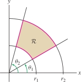
Polar coordinates are convenient when the domain of integration is an angular sector or a polar rectangle (Figure 15.42): \begin{equation*} {\mathcal{R}}: \theta_1\le \theta \le \theta_2,\quad r_1\le r \le r_2\tag{1} \end{equation*}
We assume throughout that \(r_1 \geq 0\) and that all radial coordinates are nonnegative. Recall that rectangular and polar coordinates are related by \[ x = r\cos\theta,\qquad y = r\sin \theta \]
897
Thus, we write a function \(f(x,y)\) in polar coordinates as \(f(r\cos\theta,r\sin\theta)\). The Change of Variables Formula for a polar rectangle \({\mathcal{R}}\) is: \begin{equation*} \iint_{{\mathcal{R}}\,} f(x,y)\,dA = \int_{\theta_1}^{\theta_2}\int_{r_1}^{r_2} f(r\cos\theta,r\sin\theta)\,r\,dr\,d\theta\tag{2} \end{equation*}
Eq. (2) expresses the integral of \(f(x,y)\) over the polar rectangle in Figure 15.42 as the integral of a new function \(rf(r\cos\theta,r\sin\theta)\) over the ordinary rectangle \([\theta_1,\theta_2]\times[r_1,r_2]\). In this sense, the change of variables “simplifies” the domain of integration.
Notice the extra factor \(r\) in the integrand on the right.
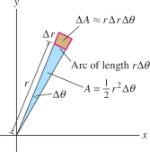
To derive Eq. (2), the key step is to estimate the area \(\Delta A\) of the small polar rectangle shown in Figure 15.43. If \(\Delta r\) and \(\Delta \theta\) are small, then this polar rectangle is very nearly an ordinary rectangle of sides \(\Delta r\) and \(r\Delta \theta\), and therefore \(\Delta A\approx r\,\Delta r\,\Delta \theta\). In fact, \(\Delta A\) is the difference of areas of two sectors: \[ \Delta A = \frac12 (r+ \Delta r)^2\,\Delta \theta - \frac12 r^2\,\Delta \theta = r(\Delta r\,\Delta \theta)+\frac12(\Delta r)^2 \Delta\theta \approx r\,\Delta r\,\Delta \theta \]
The error in our approximation is the term \(\tfrac12(\Delta r)^2 \Delta\theta\), which has smaller order of magnitude than \(\Delta r\,\Delta \theta\) when \(\Delta r\) and \(\,\Delta \theta\) are both small.
REMINDER
The length of the arc subtended by an angle \(\theta\) is \(\theta\), and the area of a sector is \(\frac12 r^2\theta\).
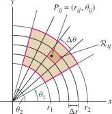
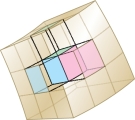
Now, decompose \({\mathcal{R}}\) into an \(N\times M\) grid of small polar subrectangles \({\mathcal{R}}_{ij}\) as in Figure 15.44, and choose a sample point \(P_{ij}\) in \({\mathcal{R}}_{ij}\). If \({\mathcal{R}}_{ij}\) is small and \(f(x,y)\) is continuous, then \begin{equation*} \iint_{{\mathcal{R}}_{ij}\,} f(x,y)\,dx\,dy \approx f(P_{ij})\,\textrm{Area}({\mathcal{R}}_{ij}) \approx f(P_{ij})\,r_{ij}\,\Delta r\,\Delta\theta\tag{3} \end{equation*}
REMINDER
In Eq. (3). we use the approximation (10) in Section 15.2: If \(f\) is continuous and \({\mathcal{D}}\) is a small domain, \[ \iint_{{\mathcal{D}}\,} f(x,y)\,dA \approx f(P)\,\textrm{Area}({\mathcal{D}}) \] where \(P\) is any sample point in \({\mathcal{D}}\).
Note that each polar rectangle \({\mathcal{R}}_{ij}\) has angular width \(\Delta \theta = (\theta_2-\theta_1)/N\) and radial width \(\Delta r=\) \((r_2-r_1)/M\). The integral over \({\mathcal{R}}\) is the sum: \[ \begin{array}{rl} \iint_{{\mathcal{R}}\,} f(x,y)\,dx\,dy &= \sum_{i=1}^N\sum_{j=1}^M \iint_{{\mathcal{R}}_{ij}\,} f(x,y)\,dx\,dy\\ &\approx \sum_{i=1}^N\sum_{j=1}^M f(P_{ij})\,\textrm{Area}({\mathcal{R}}_{ij})\\ &\approx \sum_{i=1}^N\sum_{j=1}^M f(r_{ij}\cos \theta_{ij},r_{ij}\sin \theta_{ij})\,r_{ij}\, \Delta r\,\Delta \theta \end{array} \]
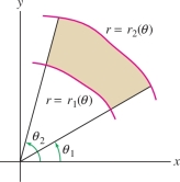
This is a Riemann sum for the double integral of \(rf(r\cos\theta,r\sin\theta)\) over the region \(r_1\le r \le r_2\), \(\theta_1\le \theta\le\theta_2\), and we can prove that it approaches the double integral as \(N,M\to\infty\). A similar derivation is valid for domains Figure 15.45 that can be described as the region between two polar curves \(r = r_1(\theta)\) and \(r = r_2(\theta)\). This gives us Theorem 1.
898
THEOREM 1 Double Integral in Polar Coordinates
For a continuous function \(f\) on the domain \[ {\mathcal{D}}: \theta_1 \le \theta \le \theta_2,\quad r_1(\theta)\le r \le r_2(\theta) \] \begin{equation*} \boxed{\iint_{{\mathcal{D}}\,} f(x,y)\,dA = \int_{\theta_1}^{\theta_2}\int_{r=r_1(\theta)}^{r_2(\theta)} f(r\cos\theta,r\sin\theta)\,r\,dr\,d\theta }\tag{4} \end{equation*}
Eq. (4) is summarized in the symbolic expression for the “area element” \(dA\) in polar coordinates: \[ \boxed{dA = r\,dr\,d\theta} \]
EXAMPLE 1
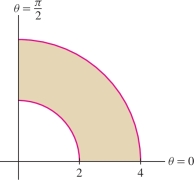
Compute \(\iint_{{\mathcal{D}}\,}(x+y)\,dA\), where \({\mathcal{D}}\) is the quarter annulus in Figure 15.46.
Solution
Step 1. Describe \({\mathcal{D}}\) and \(f\) in polar coordinates.
The quarter annulus \({\mathcal{D}}\) is defined by the inequalities Figure 15.46 \[ \displaystyle{\mathcal{D}}: 0\le\theta\le \frac{\pi}2,\quad 2\le r \le 4 \]
In polar coordinates, \[ \displaystyle f(x,y)=x+y=r\cos\theta+r\sin\theta = r(\cos\theta+\sin\theta) \]
Step 2. Change variables and evaluate.
To write the integral in polar coordinates, we replace \(dA\) by \(r\,dr\,d\theta\): \[ \iint_{{\mathcal{D}}\,}(x+y)\,dA = \int_0^{\pi/2}\int_{r=2}^4 r(\cos\theta+\sin\theta)\,r\,dr\,d\theta \]
The inner integral is \[ \int_{r=2}^4 (\cos\theta+\sin\theta)\,r^2\,dr = (\cos\theta+\sin\theta)\left(\frac{4^3}3-\frac{2^3}{3}\right) =\frac{56}3(\cos\theta+\sin\theta) \] and \[ \iint_{{\mathcal{D}}\,}(x+y)\,dA =\frac{56}3\int_0^{\pi/2}(\cos\theta+\sin\theta)\,d\theta= \frac{56}3 (\sin\theta-\cos\theta)\bigg|_0^{\pi/2} = \frac{112}3 \]
899
EXAMPLE 2
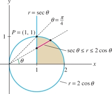
Calculate \(\iint_{{\mathcal{D}}\,}(x^2+y^2)^{-2}\,dA\) for the shaded domain \({\mathcal{D}}\) in Figure 15.47.
Solution
Step 1. Describe \({\mathcal{D}}\) and \(f\) in polar coordinates.
The quarter circle lies in the angular sector \(0\le \theta \le \frac{\pi}4\) because the line through \(P=(1,1)\) makes an angle of \(\frac{\pi}4\) with the \(x\)-axis Figure 15.47.
To determine the limits on \(r\), recall from Section 11.3 (Examples 5 and 7) that:
- The vertical line \(x=1\) has polar equation \(r\cos\theta=1\) or \(r=\sec\theta\).
- The circle of radius \(1\) and center \((1,0)\) has polar equation \(r=2\cos\theta\).
Therefore, a ray of angle \(\theta\) intersects \({\mathcal{D}}\) in the segment where \(r\) ranges from \(\sec\theta\) to \(2\cos\theta\). In other words, our domain has polar description \[ \displaystyle {\mathcal{D}}: 0\le \theta\le \frac{\pi}4,\quad \sec\theta\le r \le 2\cos\theta \]
The function in polar coordinates is \[ \displaystyle f(x,y)=(x^2+y^2)^{-2} = (r^2)^{-2} =r^{-4} \]
REMINDER
\[ \begin{array}{rl} \int \cos^2 \theta\,d\theta&=\frac12\left(\theta+\frac12\sin 2\theta\right)+C\\ \int \sec^2\theta\,d\theta &= \tan\theta +C \end{array} \]
Step 2. Change variables and evaluate.
\[ \iint_{{\mathcal{D}}\,}(x^2+y^2)^{-2}\,dA = \int_0^{\pi/4}\int_{r=\sec\theta}^{2\cos\theta} r^{-4}\,r\,dr\,d\theta = \int_0^{\pi/4}\int_{r=\sec\theta}^{2\cos\theta} r^{-3} \,dr\,d\theta \]
The inner integral is \[ \int_{r=\sec\theta}^{2\cos\theta} r^{-3} \,dr = -\frac12r^{-2}\bigg|_{r=\sec\theta}^{2\cos\theta} = - \frac18\sec^2 \theta + \frac12\cos^2 \theta \]
Therefore, \[ \begin{array}{rl} \iint_{{\mathcal{D}}\,}(x^2+y^2)^{-2}\,dA &=\int_0^{\pi/4} \left( \frac12\cos^2 \theta - \frac18\sec^2\theta \right)\,d\theta \\ &= \left(\frac14\left(\theta+\frac12\sin 2\theta\right) - \frac18\tan\theta\right) \bigg|_0^{\pi/4}\\ &= \frac14\left(\frac{\pi}4+\frac12\sin\frac{\pi}2\right)-\frac18\tan\frac{\pi}4 = \frac{\pi}{16} \end{array} \]
Triple Integrals in Cylindrical Coordinates
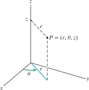
Cylindrical coordinates, introduced in Section 12.7, are useful when the domain has axial symmetry—that is, symmetry with respect to an axis. In cylindrical coordinates \((r,\theta,z)\), the axis of symmetry is the \(z\)-axis. Recall the relations Figure 15.48 \[ x =r\cos\theta,\qquad y = r\sin\theta,\qquad z = z \]
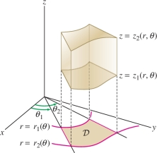
To set up a triple integral in cylindrical coordinates, we assume that the domain of integration \({\mathcal{W}}\) can be described as the region between two surfaces Figure 15.49 \[ z_1(r,\theta) \le z \le z_2(r,\theta) \] lying over a domain \({\mathcal{D}}\) in the \(xy\)-plane with polar description \[ {\mathcal{D}}: \theta_1 \le \theta \le \theta_2,\quad r_1(\theta) \le r \le r_2(\theta) \]
900
A triple integral over \({\mathcal{W}}\) can be written as an iterated integral (Theorem 2 of Section 15.3): \[ \iiint_{{\mathcal{W}}\,} f(x,y,z)\,dV = \iint_{{\mathcal{D}}\,}\left(\int_{z=z_1(r,\theta)}^{z_2(r,\theta)} f(x,y,z)\,dz\right)\,dA \]
By expressing the integral over \({\mathcal{D}}\) in polar coordinates, we obtain the following Change of Variables Formula.
Eq. (5) is summarized in the symbolic expression for the “volume element” \(dV\) in cylindrical coordinates: \[ \boxed{dV = r\,dz\,dr\,d\theta} \]
THEOREM 2 Triple Integrals in Cylindrical Coordinates
For a continuous function \(f\) on the region \[ \theta_1 \le \theta \le \theta_2,\qquad r_1(\theta) \le r \le r_2(\theta),\qquad z_1(r,\theta) \le z \le z_2(r,\theta), \] the triple integral \(\iiint_{{\mathcal{W}}\,} f(x,y,z)\,dV\) is equal to \begin{equation*} \boxed{\int_{\theta_1}^{\theta_2}\int_{r=r_1(\theta)}^{r_2(\theta)} \int_{z=z_1(r,\theta)}^{z_2(r,\theta)}f(r\cos\theta,r\sin\theta,z) \,r\,dz\,dr\,d\theta}\tag{5} \end{equation*}
EXAMPLE 3
Integrate \(f(x,y,z)=z\sqrt{x^2+y^2}\) over the cylinder \(x^2+y^2\leq 4\) for \(1 \le z \le 5\) Figure 15.50.
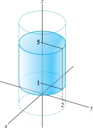
Solution The domain of integration \({\mathcal{W}}\) lies above the disk of radius \(2\), so in cylindrical coordinates, \[ {\mathcal{W}}: 0\le \theta\le 2\pi,\quad 0\le r \le 2,\quad 1\le z \le 5 \]
We write the function in cylindrical coordinates: \[ f(x,y,z)=z\sqrt{x^2+y^2}=zr \] and integrate with respect to \(dV = r\,dz\,dr\,d\theta\). The function \(f\) is a product \(zr\), so the resulting triple integral is a product of single integrals: \[ \begin{array}{rl} \iiint_{{\mathcal{W}}\,} z\sqrt{x^2+y^2}\,dV &= \int_0^{2\pi}\int_{r=0}^2\int_{z=1}^5 (zr)r\,dz\,dr\,d\theta\\ &=\left(\int_0^{2\pi} d\theta\right)\left(\int_{r=0}^2 r^2\,dr\right) \left(\int_{z=1}^5 z \,dz\right)\\ &=(2\pi)\left(\frac{2^3}3\right)\left(\frac{5^2-1^2}2\right) = 64\pi \end{array} \]
901
EXAMPLE 4
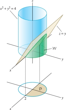
Compute the integral of \(f(x,y,z) = z\) over the region \({\mathcal{W}}\) within the cylinder \(x^2+y^2\le 4\) where \(0\le z\le y\).
Solution
Step 1. Express \({\mathcal{W}}\) in cylindrical coordinates.
The condition \(0\le z\le y\) tells us that \(y\ge 0\), so \({\mathcal{W}}\) projects onto the semicircle \({\mathcal{D}}\) in the \(xy\)-plane of radius 2 where \(y\ge 0\) shown in Figure 15.51. In polar coordinates, \[ {\mathcal{D}}: 0 \le \theta \le \pi,\quad 0\le r \le 2 \]
The \(z\)-coordinate in \({\mathcal{W}}\) varies from \(z=0\) to \(z=y\), and in polar coordinates \(y=r\sin\theta\), so the region has the description \[ {\mathcal{W}}: 0 \le \theta \le \pi,\quad 0\le r \le 2,\quad 0\le z\le r\sin\theta \]
Step 2. Change variables and evaluate.
\[ \begin{array}{rl} \iiint_{{\mathcal{W}}\,}f(x,y,z)\,dV &= \int_0^{\pi} \int_{r=0}^{2} \int_{z=0}^{r\sin\theta} zr\,dz\,dr\,d\theta \\ &= \int_0^{\pi} \int_{r=0}^{2} \frac12(r\sin\theta)^2r \,dr\,d\theta \\ &= \frac12\left(\int_0^{\pi}\sin^2\theta\,d\theta\right)\Bigg(\int_{0}^{2}r^3\,dr\Bigg) \\ &= \frac12 \left(\frac{\pi}2\right)\frac{2^4}4 = \pi \end{array} \]
REMINDER
\[ \begin{array}{rl} \int \sin^2 \theta\,d\theta &=\frac12\left(\theta -\frac12\sin 2\theta\right) +C\\ \int_0^{\pi} \sin^2 \theta\,d\theta &= \frac{\pi}2 \end{array} \]
Triple Integrals in Spherical Coordinates
We noted that the Change of Variables Formula in cylindrical coordinates is summarized by the symbolic equation \(dV=r\,dr\,d\theta\,dz\). In spherical coordinates (introduced in Section 12.7), the analog is the formula \[ \boxed{dV = \rho^2\sin\phi\,d\rho\,d\phi\, d\theta} \]
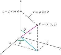
Recall Figure 15.52 that \[ x = \rho\cos\theta\sin\phi,\qquad y = \rho\sin\theta\sin\phi,\qquad z = \rho \cos\phi \]
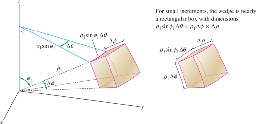
The key step in deriving this formula is estimating the volume of a small spherical wedge \({\mathcal{W}}\), defined by the inequalities \begin{equation*} {\mathcal{W}}: \theta_1\le \theta \le \theta_2,\quad \phi_1\le \phi \le \phi_2, \quad \rho_1\le \rho \le \rho_2\tag{6} \end{equation*}
902
Referring to Figure 15.53, we see that when the increments \[ \Delta \theta = \theta_2-\theta_1 ,\qquad \Delta \phi = \phi_2-\phi_1 ,\qquad \Delta \rho = \rho_2-\rho_1 \] are small, the spherical wedge is nearly a box with sides \(\Delta\rho\), \(\rho_1\Delta\phi\), and \(\rho_1\sin\phi_1\Delta\theta\) and volume \begin{equation*} \textrm{Volume}({\mathcal{W}}) \approx \rho_1^2\sin\phi_1\,\Delta\rho\,\Delta\phi\,\Delta\theta\tag{7} \end{equation*}
Following the usual steps, we decompose \({\mathcal{W}}\) into \(N^3\) spherical subwedges \({\mathcal{W}}_i\) Figure 15.54 with increments \[ \Delta \theta = \frac{\theta_2-\theta_1}N,\qquad \Delta \phi = \frac{\phi_2-\phi_1}N,\qquad \Delta \rho = \frac{\rho_2-\rho_1}N \] and choose a sample point \(P_i=(\rho_i,\theta_i,\phi_i)\) in each \({\mathcal{W}}_i\). Assuming \(f\) is continuous, the following approximation holds for large \(N\) (small \({\mathcal{W}}_i\)): \[ \begin{array}{rl} \iiint_{{\mathcal{W}}_i\,} f(x,y,z)\,dV &\approx f(P_i)\textrm{Volume}({\mathcal{W}}_i)\\ &\approx f(P_i)\rho_i^2\sin\phi_i\,\Delta\rho\,\Delta\theta\,\Delta\phi \end{array} \]
Taking the sum over \(i\), we obtain \begin{equation*} \iiint_{{\mathcal{W}}\,} f(x,y,z)\,dV \approx \sum_{i} f(P_i)\rho_i^2\sin\phi_i\,\Delta\rho\, \Delta\theta\, \Delta\phi\tag{8} \end{equation*}
The sum on the right is a Riemann sum for the function \[ f(\rho\cos\theta\sin\phi,\rho\sin\theta\sin\phi,\rho\cos\phi)\,\rho^2\sin\phi \] on the domain \({\mathcal{W}}\). Eq. (9) below follows by passing to the limit an \(N \to \infty\) (and showing that the error in Eq. (8) tends to zero). This argument applies more generally to regions defined by an inequality \(\rho_1(\theta,\phi)\le \rho \le \rho_2(\theta,\phi)\).
903
THEOREM 3 Triple Integrals in Spherical Coordinates
For a region \({\mathcal{W}}\) defined by \[ \theta_1 \le \theta \le \theta_2,\qquad \phi_1 \le \phi \le\phi_2,\qquad \rho_1(\theta,\phi)\le \rho \le \rho_2(\theta,\phi) \] the triple integral \(\iiint_{{\mathcal{W}}\,} f(x,y,z)\,dV\) is equal to \begin{equation*} \boxed{\int_{\theta_1}^{\theta_2}\int_{\phi = \phi_1}^{\phi_2}\int_{\rho = \rho_1(\theta,\phi)}^{\rho_2(\theta,\phi)} f(\rho\cos\theta\sin\phi,\rho\sin\theta\sin\phi,\rho\cos\phi)\, \rho^2\sin\phi\,d\rho\,d\phi\,d\theta }\tag{9} \end{equation*}
Eq. (9) is summarized in the symbolic expression for the “volume element” \(dV\) in spherical coordinates: \[ \boxed{dV = \rho^2\,\sin\phi\,d\rho\,d\phi\,d\theta} \]
EXAMPLE 5
Compute the integral of \(f(x,y,z)=x^2+y^2\) over the sphere \(S\) of radius \(4\) centered at the origin Figure 15.55.
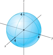
Solution First, write \(f(x,y,z)\) in spherical coordinates: \[ \begin{array}{rl} f(x,y,z)&=x^2+y^2 = (\rho\cos\theta\sin\phi)^2 + (\rho\sin\theta\sin\phi)^2 \\ &=\rho^2\sin^2\phi(\cos^2\theta+\sin^2\theta)=\rho^2\sin^2\phi \end{array} \]
Since we are integrating over the entire sphere \(S\) of radius 4, \(\rho\) varies from 0 to 4, \(\theta\) from 0 to \(2\pi\), and \(\phi\) from 0 to \(\pi\). In the following computation, we integrate first with respect to \(\theta\): \[ \begin{array}{rl} \iiint_{S\,}(x^2+y^2)\,dV &=\int_0^{2\pi}\int_{\phi = 0}^{\pi}\int_{\rho=0}^4 (\rho^2\sin^2\phi)\,\rho^2\sin\phi\,d\rho\,d\phi\,d\theta\\ &= 2\pi \int_{\phi = 0}^{\pi}\int_{\rho = 0}^4 \rho^4\sin^3\phi \,d\rho\,d\phi = 2\pi \int_0^{\pi} \left(\frac{\rho^5}5 \bigg|_0^4\right) \sin^3 \phi \,d\phi\\ &= \frac{2048\pi}{5}\int_0^{\pi} \sin^3\phi \,d\phi\\ &= \frac{2048\pi}{5}\left(\frac13\cos^3\phi -\cos\phi\right)\bigg|_0^{\pi} =\frac{8192\pi}{15} \end{array} \]
REMINDER
\[ \int\sin^3\phi\,d\phi = \frac13\cos^3\phi -\cos\phi+C \] [write \(\sin^3\phi=\sin\phi(1-\cos^2\phi)\)]
EXAMPLE 6
Integrate \(f(x,y,z)=z\) over the ice cream cone–shaped region \({\mathcal{W}}\) in Figure 15.56, lying above the cone and below the sphere.
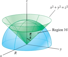
Solution The cone has equation \(x^2+y^2=z^2\), which in spherical coordinates is \[ \begin{array}{rl} (\rho\cos\theta\sin\phi)^2+(\rho\sin\theta\sin\phi)^2 &= (\rho\cos \phi)^2 \\ \rho^2\sin^2\phi(\cos^2\theta + \sin^2\theta) &= \rho^2\cos^2 \phi\\ \sin^2\phi &= \cos^2\phi\\ \sin\phi &= \pm\cos \phi\quad\Rightarrow\quad \phi = \frac{\pi}4, \frac{3\pi}4 \end{array} \]
The upper branch of the cone has the simple equation \(\phi=\frac{\pi}4\). On the other hand, the sphere has equation \(\rho = R\), so the ice cream cone has the description \[ {\mathcal{W}}: 0\le\theta\le 2\pi ,\quad 0\le \phi\le\frac{\pi}4,\quad 0 \le \rho \le R \]
904
We have \[ \begin{array}{rl} \iiint_{{\mathcal{W}}\,} z \,dV &= \int_0^{2\pi}\int_{\phi=0}^{\pi/4}\int_{\rho = 0}^R (\rho\cos\phi)\rho^2\sin\phi\,d\rho\,d\phi\,d\theta\\ &= 2\pi\int_{\phi=0}^{\pi/4}\int_{\rho = 0}^R \rho^3\cos\phi \sin\phi\,d\rho\,d\phi = \frac{\pi R^4}2 \int_{0}^{\pi/4} \sin \phi\cos\phi \, d\phi = \frac{\pi R^4}8 \end{array} \]
15.4.1 Summary
In symbolic form: \[ \boxed{dA = r\,dr\,d\theta} \] \[ \boxed{dV = r\,dz\,dr\,d\theta} \] \[ \boxed{dV = \rho^2\sin\phi\,d\rho\,d\phi\,d\theta} \]
- Double integral in polar coordinates: \[ \iint_{{\mathcal{D}}\,} f(x,y)\,dA = \int_{\theta_1}^{\theta_2}\int_{r=r_1(\theta)}^{r_2(\theta)}\, f(r\cos\theta,r\sin\theta)\,r\,dr\,d\theta \]
- Triple integral \(\iiint_{{\mathcal{R}}\,}f(x,y,z)\,dV\)
- – In cylindrical coordinates: \[ \int_{\theta_1}^{\theta_2}\int_{r=r_1(\theta)}^{r_2(\theta)} \int_{z=z_1(r,\theta)}^{z_2(r,\theta)}f(r\cos\theta,r\sin\theta,z)\,r\,dz\,dr\,d\theta \]
- – In spherical coordinates: \[ \int_{\theta_1}^{\theta_2} \int_{\phi = \phi_1}^{\phi_2}\int_{\rho = \rho_1(\theta,\phi)}^{\rho_2(\theta,\phi)} f(\rho\cos\theta\sin\phi,\rho\sin\theta\sin\phi,\rho\cos\phi)\,\rho^2\sin\phi\,d\rho\,d\phi\,d\theta \]