16.2 Line Integrals
In this section we introduce two types of integrals over curves: integrals of functions and integrals of vector fields. These are traditionally called line integrals, although it would be more appropriate to call them “curve” or “path” integrals.
Scalar Line Integrals
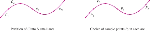
We begin by defining the scalar line integral \(\int_{{\mathcal{C}}} f(x,y,z)\,ds\) of a function \(f\) over a curve \({\mathcal{C}}\). We will see how integrals of this type represent total mass and charge, and how they can be used to find electric potentials. Like all integrals, this line integral is defined through a process of subdivision, summation, and passage to the limit. We divide \({\mathcal{C}}\) into \(N\) consecutive arcs \({\mathcal{C}}_1, \ldots, {\mathcal{C}}_N\), choose a sample point \(P_i\) in each arc \({\mathcal{C}}_i\), and form the Riemann sum (Figure 16.10) \[ \sum_{i=1}^N f(P_i)\,\textrm{length(}{\mathcal{C}}_i) = \sum_{i=1}^N f(P_i)\,\Delta s_i \] where \(\Delta s_i\) is the length of \({\mathcal{C}}_i\).
947
The line integral of \(f\) over \({\mathcal{C}}\) is the limit (if it exists) of these Riemann sums as the maximum of the lengths \(\Delta s_i\) approaches zero: \begin{equation*} \boxed{\int_{\mathcal{C}} f(x,y,z)\,ds = \lim_{\{\Delta s_i\}\to 0} \sum_{i=1}^N f(P_i)\,\Delta s_i }\tag{1} \end{equation*}
In Eq. (1), we write \(\{\Delta s_i\}\to 0\) to indicate that the limit is taken over all Riemann sums as the maximum of the lengths \(\Delta s_i\) tends to zero.
This definition also applies to functions \(f(x,y)\) of two variables. The scalar line integral of the function \(f(x,y,z)=1\) is simply the length of \({\mathcal{C}}\). In this case, all the Riemann sums have the same value: \[ \sum_{i=1}^N 1\,\Delta s_i = \sum_{i=1}^N \textrm{length}({\mathcal{C}}_i) = \textrm{length}({\mathcal{C}}) \] and thus \[ \boxed{\int_{\mathcal{C}} 1\,ds = \textrm{length}({\mathcal{C}})} \]
In practice, line integrals are computed using parametrizations. Suppose that \({\mathcal{C}}\) has a parametrization \({\bf{c}}(t)\) for \(a \leq t \leq b\) with continuous derivative \({\bf{c}}'(t)\). Recall that the derivative is the tangent vector \[ {\bf{c}}'(t) = \left\langle x'(t), y'(t), z'(t)\right\rangle \]
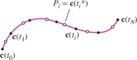
We divide \({\mathcal{C}}\) into \(N\) consecutive arcs \({\mathcal{C}}_1, \ldots, {\mathcal{C}}_N\) corresponding to a partition of the interval \([a,b]\): \[ a = t_0 < t_1 < \cdots < t_{N-1} < t_N = b \] so that \({\mathcal{C}}_i\) is parametrized by \({\bf{c}}(t)\) for \(t_{i-1} \le t \le t_i\) (Figure 16.11), and choose sample points \(P_i={\bf{c}}(t_i^{*})\) with \(t_i^{*}\) in \([t_{i-1},t_i]\). According to the arc length formula (Section 13.3), \[ \textrm{Length(}{\mathcal{C}}_i) = \Delta s_i = \int_{t_{i-1}}^{t_i} \left \| {{\bf{c}}'(t)} \right \|\,dt \]
Because \({\bf{c}}'(t)\) is continuous, the function \(\left \| {{\bf{c}}'(t)} \right \|\) is nearly constant on \([t_{i-1},t_i]\) if the length \(\Delta t_i =t_i - t_{i-1}\) is small, and thus \(\int_{t_{i-1}}^{t_i} \left \| {{\bf{c}}'(t)} \right \|\,dt\approx \left \|{{\bf{c}}'(t_i^{*})} \right \|\Delta t_i\). This gives us the approximation \begin{equation*} \sum_{i=1}^N f(P_i)\,\Delta s_i \approx \sum_{i=1}^N f({\bf{c}}(t_i^*)) \left \| {{\bf{c}}'(t_i^{*})} \right \|\,\Delta t_i\tag{2} \end{equation*}
REMINDER
Arc length formula: The length \(s\) of a path \({\bf{c}}(t)\) for \(a\le t\le b\) is \[ s = \int_a^b \left \| {{\bf{c}}'(t)} \right \|\, dt \]
948
The sum on the right is a Riemann sum that converges to the integral \begin{equation*} \int_a^b f({\bf{c}}(t))\left \| {{\bf{c}}'(t)} \right \|\,dt\tag{3} \end{equation*} as the maximum of the lengths \(\Delta t_i\) tends to zero. By estimating the errors in this approximation, we can show that the sums on the left-hand side of (2) also approach (3). This gives us the following formula for the scalar line integral.
THEOREM 1 Computing a Scalar Line Integral
Let \({\bf{c}}(t)\) be a parametrization of a curve \({\mathcal{C}}\) for \(a\le t\le b\). If \(f(x,y,z)\) and \({\bf{c}}'(t)\) are continuous, then \begin{equation*} \boxed{\int_{\mathcal{C}} f(x,y,z)\,ds = \int_a^b f({\bf{c}}(t))\left \| {{\bf{c}}'(t)} \right \|\,dt}\tag{4} \end{equation*}
The symbol \(ds\) is intended to suggest arc length \(s\) and is often referred to as the line element or arc length differential. In terms of a parametrization, we have the symbolic equation \[ \boxed{ds = \left \| {{\bf{c}}'(t)} \right \|\,dt} \] where \[ \left \| {{\bf{c}}'(t)} \right \| = \sqrt{x'(t)^2+y'(t)^2+z'(t)^2} \]
Eq. (4) tells us that to evaluate a scalar line integral, we replace the integrand \(f(x,y,z)\,ds\) with \(f({\bf{c}}(t))\,\left \| {{\bf{c}}'(t)} \right \|\,dt\).
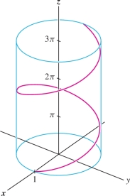
EXAMPLE 1 Integrating along a Helix
Calculate \[ \int_{\mathcal{C}} (x+y+z)\,ds \] where \({\mathcal{C}}\) is the helix \({\bf{c}}(t) = (\cos t, \sin t, t)\) for \(0\le t \le \pi\) (Figure 16.12).
Solution
Step 1. Compute \(ds\).
\[ \begin{array}{rl} {\bf{c}}'(t) &= \left\langle -\sin t, \cos t, 1\right\rangle\\ \left \| {{\bf{c}}'(t)} \right \| &= \sqrt{(-\sin t)^2+\cos^2t+1}=\sqrt 2\\ ds &= \left \| {{\bf{c}}'(t)} \right \| dt = \sqrt 2\,dt \end{array} \]
Step 2. Write out the integrand and evaluate.
We have \(f(x,y,z) = x + y + z\), and so \[ \begin{array}{rl} f({\bf{c}}(t)) &= f(\cos t,\sin t, t) = \cos t+\sin t+t\\ f(x,y,z)\,ds &= f({\bf{c}}(t))\,\left \| {{\bf{c}}'(t)} \right \|\,dt = ( \cos t+\sin t+t)\sqrt 2\,dt \end{array} \]
949
By Eq. (4), \[ \begin{array}{rl} \int_{{\mathcal{C}}} f(x,y,z)\,ds &= \int_0^\pi f({\bf{c}}(t))\,\left \| {{\bf{c}}'(t)} \right \|\,dt = \int_0^{\pi} (\cos t+\sin t + t)\sqrt{2} \,dt \\ &= \sqrt{2}\left(\sin t-\cos t + \frac12t^2\right)\bigg|_0^{\pi}\\ &= \sqrt{2}\left(0+1+\frac12\pi^2\right)-\sqrt{2}\,(0-1+0) = 2\sqrt{2}+ \frac{\sqrt{2}}2\pi^2 \end{array} \]
EXAMPLE 2 Arc Length
Calculate \(\int_{\mathcal{C}} 1\,ds\) for the helix in the previous example: \({\bf{c}}(t) = (\cos t, \sin t, t)\) for \(0\le t \le \pi\). What does this integral represent?
Solution In the previous example, we showed that \(ds = \sqrt 2\,dt\) and thus \[ \int_{{\mathcal{C}}} 1\,ds = \int_0^\pi \sqrt{2} \,dt = \pi\sqrt{2} \]
This is the length of the helix for \(0\le t \le \pi\).
Applications of the Scalar Line Integral
In Section 15.5 we discussed the general principle that “the integral of a density is the total quantity.” This applies to scalar line integrals. For example, we can view the curve \({\mathcal{C}}\) as a wire with continuous mass density \(\rho(x,y,z)\), given in units of mass per unit length. The total mass is defined as the integral of mass density: \begin{equation*} \boxed{\textrm{Total mass of }{\mathcal{C}} = \int_{\mathcal{C}}\,\rho(x,y,z)\,ds}\tag{5} \end{equation*}
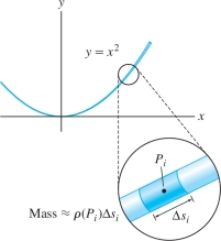
A similar formula for total charge is valid if \(\rho(x,y,z)\) is the charge density along the curve. As in Section 15.5, we justify this interpretation by dividing \({\mathcal{C}}\) into \(N\) arcs \({\mathcal{C}}_i\) of length \(\Delta s_i\) with \(N\) large. The mass density is nearly constant on \({\mathcal{C}}_i\), and therefore, the mass of \({\mathcal{C}}_i\) is approximately \(\rho(P_i)\,\Delta s_i\), where \(P_i\) is any sample point on \({\mathcal{C}}_i\) (Figure 16.13). The total mass is the sum \[ \textrm{Total mass of }{\mathcal{C}} = \sum_{i=1}^N \textrm{mass of }{\mathcal{C}}_i \approx \sum_{i=1}^N \rho(P_i)\,\Delta s_i \]
As the maximum of the lengths \(\Delta s_i\) tends to zero, the sums on the right approach the line integral in Eq. (5).
EXAMPLE 3 Scalar Line Integral as Total Mass
Find the total mass of a wire in the shape of the parabola \(y=x^2\) for \(1\le x\le 4\) (in centimeters) with mass density given by \(\rho(x,y)=y/x\)~g/cm.
Solution The arc of the parabola is parametrized by \({\bf{c}}(t)=(t,t^2)\) for \(1\le t\le 4\).
Step 1. Compute \(ds\).
\[ \begin{array}{rl} {\bf{c}}'(t) &= \left\langle 1, 2t\right\rangle\\ ds&= \left \| {{\bf{c}}'(t)} \right \|\,dt = \sqrt{1+4t^2}\,dt \end{array} \]
950
Step 2. Write out the integrand and evaluate.
We have \(\rho({\bf{c}}(t)) = \rho(t,t^2) = t^2/t=t\), and thus \[ \rho(x,y)\,ds = \rho({\bf{c}}(t))\sqrt{1+4t^2}\,dt = t\sqrt{1+4t^2}\,dt \]
We evaluate the line integral of mass density using the substitution \(u=1+4t^2\), \(du = 8t\,dt\): \[ \begin{array}{rl} \int_{\mathcal{C}} \rho(x,y)\,ds &= \int_1^4 \rho({\bf{c}}(t))\left \| {{\bf{c}}'(t)} \right \|\,dt = \int_1^{4}\ t\sqrt{1+4t^2}\,dt\\ & = \frac18 \int_5^{65}\sqrt{u}\,du = \frac1{12} u^{3/2}\bigg|_5^{65} \\ &= \frac1{12}(65^{3/2} - 5^{3/2}) \approx 42.74 \end{array} \]
Note that after the substitution, the limits of integration become \(u(1)=5\) and \(u(4)=65\). The total mass of the wire is approximately 42.7 g.
Scalar line integrals are also used to compute electric potentials. When an electric charge is distributed continuously along a curve \({\mathcal{C}}\), with charge density \(\rho(x,y,z)\), the charge distribution sets up an electrostatic field \({\bf{E}}\) that is a conservative vector field. Coulomb’s Law tells us that \({\bf{E}} = -\nabla{V}\) where \begin{equation*} \boxed{{V}(P) = k\int_{\mathcal{C}} \frac{\rho(x,y,z)\,ds}{r_P}}\tag{6} \end{equation*}
By definition, \({\bf{E}}\) is the vector field with the property that the electrostatic force on a point charge \(q\) placed at location \(P = (x,y,z)\) is the vector \(q{\bf{E}}(x,y,z)\).
In this integral, \(r_P=r_P(x,y,z)\) denotes the distance from \((x,y,z)\) to \(P\). The constant \(k\) has the value \(k = 8.99\times 10^9\) N-m\(^2\)/C\(^2\). The function \({V}\) is called the electric potential. It is defined for all points \(P\) that do not lie on \({\mathcal{C}}\) and has units of volts (one volt is one N-m/C).
The constant \(k\) is usually written as \(\frac1{4\pi\epsilon_0}\) where \(\epsilon_0\) is the vacuum permittivity.
EXAMPLE 4 Electric Potential
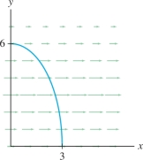
A charged semicircle of radius \(R\) centered at the origin in the \(xy\)-plane (Figure 16.14) has charge density \[ \rho(x,y,0) = 10^{-8}\left(2-\frac{x}{R}\right)\,\, \textrm{C/m} \] Find the electric potential at a point \(P=(0,0,a)\) if \(R = 0.1\) m.
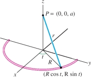
Solution Parametrize the semicircle by \({\bf{c}}(t) = (R\cos t, R\sin t, 0)\) for \(-\pi/2\le t\le \pi/2\): \[ \begin{array}{rl} \|{\bf{c}}'(t)\| &= \left \| {\left\langle -R\sin t, R\cos t, 0\right\rangle} \right \| = \sqrt{R^2\sin^2t+R^2\cos^2t+0} = R\\ ds &= \left \| {{\bf{c}}'(t)} \right \|\,dt = R\,dt\\ \rho({\bf{c}}(t)) &= \rho(R\cos t, R\sin t, 0) = 10^{-8}\left(2- \frac{R\cos t}R\right) = 10^{-8}(2-\cos t) \end{array} \]
In our case, the distance \(r_P\) from \(P\) to a point \((x,y,0)\) on the semicircle has the constant value \(r_P = \sqrt{R^2+a^2}\) (Figure 16.14). Thus, \[ \begin{array}{rl} {V}(P) &= k\int_{\mathcal{C}} \frac{\rho(x,y,z)\,ds}{r_P} = k\int_{\mathcal{C}} \frac{10^{-8}(2-\cos t)\,Rdt}{\sqrt{R^2+a^2}} \\ &= \frac{10^{-8}kR}{\sqrt{R^2+a^2}}\int_{-\pi/2}^{\pi/2} (2-\cos t)\,dt =\frac{10^{-8}kR}{\sqrt{R^2+a^2}}(2\pi-2) \end{array} \]
951
With \(R=0.1\) m and \(k = 8.99\times 10^9\), we then obtain \(10^{-8}kR(2\pi-2)\approx 38.5\) and \({V}(P) \approx \frac{38.5}{\sqrt{0.01+a^2}}\) volts.
Vector Line Integrals
When you carry a backpack up a mountain, you do work against the Earth’s gravitational field. The work, or energy expended, is one example of a quantity represented by a vector line integral.
An important difference between vector and scalar line integrals is that vector line integrals depend on a direction along the curve. This is reasonable if you think of the vector line integral as work, because the work performed going down the mountain is the negative of the work performed going up.
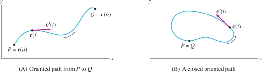
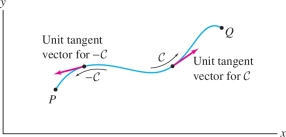
A specified direction along a path curve \({\mathcal{C}}\) is called an orientation (Figure 16.15). We refer to this direction as the positive direction along \({\mathcal{C}}\), the opposite direction is the negative direction, and \({\mathcal{C}}\) itself is called an oriented curve. In Figure 16.15, if we reversed the orientation, the positive direction would become the direction from \(Q\) to \(P\).
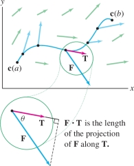
The line integral of a vector field \({\bf{F}}\) over a curve \({\mathcal{C}}\) is defined as the scalar line integral of the tangential component of \({\bf{F}}\). More precisely, let \({\bf{T}} = {\bf{T}}(P)\) denote the unit tangent vector at a point \(P\) on \({\mathcal{C}}\) pointing in the positive direction. The tangential component of \({\bf{F}}\) at \(P\) is the dot product (Figure 16.16) \[ {\bf{F}}(P) \cdot {\bf{T}}(P) = \left \| {{\bf{F}}(P)} \right \|\,\left \| {{\bf{T}}(P)} \right \| \cos\theta = \left \| {{\bf{F}}(P)} \right \| \cos\theta \] where \(\theta\) is the angle between \({\bf{F}}(P)\) and \({\bf{T}}(P)\). The vector line integral of~\({\bf{F}}\) is the scalar line integral of the scalar function \({\bf{F}}{\cdot}{\bf{T}}\) . We make the standing assumption that \({\mathcal{C}}\) is piecewise smooth (it consists of finitely many smooth curves joined together with possible corners).
The unit tangent vector \({\bf{T}}\) varies from point to point along the curve. When it is necessary to stress this dependence, we write \({\bf{T}}(P)\).
DEFINITION Vector Line Integral
The line integral of a vector field \({\bf{F}}\) along an oriented curve \({\mathcal{C}}\) is the integral of the tangential component of \({\bf{F}}\): \begin{equation*} \int_{\mathcal{C}} {\bf{F}}{\cdot}\,d{\bf{s}} = \int_{\mathcal{C}} ({\bf{F}}{\cdot}{\bf{T}})\,ds\tag{7} \end{equation*}
We use parametrizations to evaluate vector line integrals, but there is one important difference with the scalar case: The parametrization \({\bf{c}}(t)\) must be positively oriented; that is, \({\bf{c}}(t)\) must trace \({\mathcal{C}}\) in the positive direction. We assume also that \({\bf{c}}(t)\) is regular; that is, \({\bf{c}}'(t)\ne \mathbf{0}\) for \(a\le t\le b\). Then \({\bf{c}}'(t)\) is a nonzero tangent vector pointing in the positive direction, and \[ {\bf{T}} = \frac{{\bf{c}}'(t)}{\left \| {{\bf{c}}'(t)} \right \|} \]
952
In terms of the arc length differential \(ds = \left \| {{\bf{c}}'(t)} \right \|\,dt\), we have \[ ({\bf{F}}{\cdot}{\bf{T}})\,ds = \left({\bf{F}}({\bf{c}}(t)){\cdot}\frac{{\bf{c}}'(t)}{\left \| {{\bf{c}}'(t)} \right \|}\right) \left \| {{\bf{c}}'(t)} \right \|\,dt = {\bf{F}}({\bf{c}}(t)){\cdot} {\bf{c}}'(t) \,dt \]
Therefore, the integral on the right-hand side of Eq. (7) is equal to the right-hand side of Eq. (8) in the next theorem.
THEOREM 2 Computing a Vector Line Integral
If \({\bf{c}}(t)\) is a regular parametrization of an oriented curve \({\mathcal{C}}\) for \(a\le t\le b\), then \begin{equation*} \boxed{ \int_{\mathcal{C}} {\bf{F}}{\cdot}\,d{\bf{s}} = \int_a^b {\bf{F}}({\bf{c}}(t)){\cdot}{\bf{c}}'(t)\,dt}\tag{8} \end{equation*}
It is useful to think of \(d{\bf{s}}\) as a “vector line element” or “vector differential” that is related to the parametrization by the symbolic equation \[ \boxed{d{\bf{s}}={\bf{c}}'(t)\,dt} \]
Eq. (8) tells us that to evaluate a vector line integral, we replace the integrand \({\bf{F}}{\cdot}\,d{\bf{s}}\) with \({\bf{F}}({\bf{c}}(t)){\cdot}{\bf{c}}'(t)\,dt\).
Vector line integrals are usually easier to calculate than scalar line integrals, because the length \(\left \| {{\bf{c}}'(t)} \right \|\), which involves a square root, does not appear in the integrand.
EXAMPLE 5
Evaluate \(\int_{\mathcal{C}} {\bf{F}}{\cdot}\,d{\bf{s}}\), where \({\bf{F}}=\big\langle z,y^2,x \big\rangle\) and \({\mathcal{C}}\) is parametrized (in the positive direction) by \({\bf{c}}(t)=(t+1,e^t, t^2)\) for \(0\le t \le 2\).
Solution There are two steps in evaluating a line integral.
Step 1. Calculate the integrand.
\[ \begin{array}{rl} {\bf{c}}(t)&=(t+1,e^t, t^2)\\ {\bf{F}}({\bf{c}}(t)) &= \big\langle z, y^2, x \big\rangle = \big\langle t^2,e^{2t},t+1 \big\rangle\\ {\bf{c}}'(t) &= \big\langle 1,e^t, 2t\big\rangle \end{array} \]
The integrand (as a differential) is the dot product: \[ {\bf{F}}({\bf{c}}(t)){\cdot} {\bf{c}}'(t)dt = \big\langle t^2,e^{2t},t+1 \big\rangle{\cdot}\big\langle 1,e^t, 2t\big\rangle \,dt = (e^{3t}+3t^2+2t)dt \]
Step 2. Evaluate the line integral.
\[ \begin{array}{rl} \int_{\mathcal{C}} {\bf{F}}{\cdot}\,d{\bf{s}} &= \int_0^2 {\bf{F}}({\bf{c}}(t)) \cdot {\bf{c}}'(t)\,dt \\ &=\int_0^2(e^{3t}+3t^2+2t)\,dt = \left(\frac13 e^{3t} + t^3 + t^2\right)\bigg|_0^2 \\ &=\left(\frac13e^6+8+4\right)-\frac13 = \frac13\left(e^6+35\right) \end{array} \]
Another standard notation for the line integral \(\int_{\mathcal{C}} {\bf{F}}{\cdot}\,d{\bf{s}}\) is \[ \boxed{\int_{\mathcal{C}} F_1\, dx + F_2\, dy + F_3\, dz} \]
953
In this notation, we write \(d{\bf{s}}\) as a vector differential \[ d{\bf{s}} = \left\langle dx, dy, dz\right\rangle \] so that \[ {\bf{F}}{\cdot}\,d{\bf{s}} = \left\langle F_1, F_2, F_3\right\rangle{\cdot} \left\langle dx, dy, dz\right\rangle = F_1\, dx + F_2\, dy + F_3\, dz \]
In terms of a parametrization \({\bf{c}}(t)=\left(x(t),y(t),z(t)\right)\), \[ \begin{array}{rl} d{\bf{s}} &= \left\langle \frac{d x}{d t}, \frac{d y}{d t}, \frac{d z}{d t}\right\rangle\,dt\\ {\bf{F}}{\cdot}\,d{\bf{s}} &= \left(F_1({\bf{c}}(t))\frac{d x}{d t} + F_2({\bf{c}}(t))\frac{d y}{d t} + F_3({\bf{c}}(t))\frac{d z}{d t}\right) \, dt \end{array} \]
So we have the following formula: \[ \boxed{\int_{\mathcal{C}} F_1\, dx + F_2\, dy + F_3\, dz=\int_a^b \left(F_1({\bf{c}}(t))\frac{d x}{d t} +F_2({\bf{c}}(t))\frac{d y}{d t} +F_3({\bf{c}}(t))\frac{d z}{d t}\right) \, dt} \]
GRAPHICAL INSIGHT
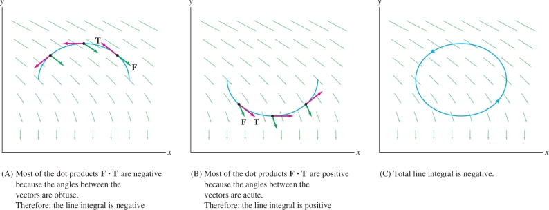
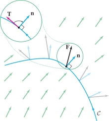
The magnitude of a vector line integral (or even whether it is positive or negative) depends on the angles between \({\bf{F}}\) and \({\bf{T}}\) along the path. Consider the line integral of \({\bf{F}}= \left\langle 2y, -3\right\rangle\) around the ellipse in Figure 16.17.
- In Figure 16.17, the angles \(\theta\) between \({\bf{F}}\) and \({\bf{T}}\) appear to be mostly obtuse along the top part of the ellipse. Consequently, \({\bf{F}}{\cdot}{\bf{T}} \le 0\) and the line integral is negative.
- In Figure 16.17, the angles \(\theta\) appear to be mostly acute along the bottom part of the ellipse. Consequently, \({\bf{F}}{\cdot}{\bf{T}} \ge 0\) and the line integral is positive.
- We can guess that the line integral around the entire ellipse is negative because \(\left \| {\bf{F}} \right \|\) is larger in the top half, so the negative contribution of \({\bf{F}}{\cdot}{\bf{T}}\) from the top half appears to dominate the positive contribution of the bottom half. We verify this in Example 6.
954
EXAMPLE 6
The ellipse \({\mathcal{C}}\) in Figure 16.17 with counterclockwise orientation is parametrized by \({\bf{c}}(\theta)=(5+4\cos\theta,3+2\sin\theta)\) for \(0 \le \theta < 2\pi\). Calculate \[ \int_{{\mathcal{C}}} 2y\,dx-3\,dy \]
Solution We have \(x(\theta)=5+4\cos\theta\) and \(y(\theta) = 3+2\sin\theta\), and \[ \frac{d x}{d \theta} = -4\sin\theta,\qquad \frac{d y}{d \theta} = 2\cos\theta \]
In Example 6, keep in mind that \[ \int_{\mathcal{C}}\, 2y\,dx - 3\,dy \] is another notation for the line integral of \({\bf{F}}=\left\langle 2y,-3\right\rangle\) over \({\mathcal{C}}\). Formally, \[ \begin{array}{rl} {\bf{F}}{\cdot}\,d{\bf{s}}&=\left\langle 2y,-3\right\rangle{\cdot}\left\langle dx,dy\right\rangle\\ & = 2y\,dx - 3\,dy \end{array} \]
The integrand of the line integral is \[ \begin{array}{rcl} 2y\,dx-3\,dy &=& \left(2y\frac{d x}{d \theta} - 3\frac{d y}{d \theta}\right)d\theta\\ &=& \bigl(2(3+2\sin\theta)(-4\sin\theta) - 3(2\cos\theta)\bigr)\,d\theta\\ &=& -\bigl(24\sin\theta + 16\sin^2\theta + 6\cos\theta\bigr)\,d\theta \end{array} \]
Since the integrals of \(\cos\theta\) and \(\sin\theta\) over \([0,2\pi]\) are zero, \[ \begin{array}{rcl} \int_{\mathcal{C}} 2y\,dx - 3\,dy &=& -\int_0^{2\pi} \bigl(24\sin\theta + 16\sin^2\theta + 6\cos\theta\bigr)\,d\theta \\ &=& -16 \int_0^{2\pi} \sin^2\theta\,d\theta = -16\pi \end{array} \]
REMINDER
- \(\int\sin^2\theta\,d\theta = \frac12\theta-\frac14\sin2\theta\)
- \(\int_0^{2\pi}\sin^2\theta\,d\theta = \pi\)
We now state some basic properties of vector line integrals. First, given an oriented curve \({\mathcal{C}}\), we write \(-{\mathcal{C}}\) to denote the curve \({\mathcal{C}}\) with the opposite orientation (Figure 16.18). The unit tangent vector changes sign from \({\bf{T}}\) to \(-{\bf{T}}\) when we change orientation, so the tangential component of \({\bf{F}}\) and the line integral also change sign: \[ \int_{-{\mathcal{C}}} {\bf{F}}{\cdot} d{\bf{s}} = -\int_{\mathcal{C}}{\bf{F}}{\cdot} d{\bf{s}} \]
Next, if we are given \(n\) oriented curves \({\mathcal{C}}_1,\ldots,{\mathcal{C}}_n\), we write \[ {\mathcal{C}} = {\mathcal{C}}_1 + \cdots + {\mathcal{C}}_n \] to indicate the union of the paths, and we define the line integral over \({\mathcal{C}}\) as the sum \[ \int_{\mathcal{C}} {\bf{F}}{\cdot}\,d{\bf{s}} = \int_{{\mathcal{C}}_1} {\bf{F}}{\cdot}\,d{\bf{s}}+\cdots + \int_{{\mathcal{C}}_n} {\bf{F}}{\cdot}\,d{\bf{s}} \]
We use this formula to define the line integral when \({\mathcal{C}}\) is piecewise smooth, meaning that \({\mathcal{C}}\) is a union of smooth curves \({\mathcal{C}}_1,\ldots,{\mathcal{C}}_n\). For example, the triangle in Figure 16.19 is piecewise smooth but not smooth. The next theorem summarizes the main properties of vector line integrals.
955
THEOREM 3 Properties of Vector Line Integrals
Let \({\mathcal{C}}\) be a smooth oriented curve, and let \({\bf{F}}\) and \({\bf{G}}\) be vector fields.
- (i) Linearity: \(\begin{array}{l} \displaystyle\int_{\mathcal{C}} ({\bf{F}} + {\bf{G}}) {\cdot} d{\bf{s}} = \int_{\mathcal{C}} {\bf{F}} {\cdot} d{\bf{s}}+\int_{\mathcal{C}} {\bf{G}} {\cdot} d{\bf{s}}\\ \displaystyle \int_{\mathcal{C}} k{\bf{F}} {\cdot} d{\bf{s}} = k \int_{\mathcal{C}} {\bf{F}}{\cdot} d{\bf{s}}\quad (k\textrm{ a constant)} \end{array}\)
- (ii) Reversing orientation: \(\int_{-{\mathcal{C}}}{\bf{F}}{\cdot} d{\bf{s}} = -\int_{\mathcal{C}}{\bf{F}}{\cdot} d{\bf{s}}\)
- (iii) Additivity: If \({\mathcal{C}}\) is a union of \(n\) smooth curves \({\mathcal{C}}_1+\cdots+{\mathcal{C}}_n\), then \[ \int_{\mathcal{C}} {\bf{F}}{\cdot} d{\bf{s}} = \int_{{\mathcal{C}}_1} {\bf{F}}{\cdot} d{\bf{s}}+\cdots + \int_{{\mathcal{C}}_n} {\bf{F}}{\cdot} d{\bf{s}} \]
EXAMPLE 7
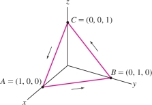
Compute \(\int_{\mathcal{C}}{\bf{F}} {\cdot} d{\bf{s}}\), where \({\bf{F}} = \left\langle e^z, e^y, x+y\right\rangle\) and \({\mathcal{C}}\) is the triangle joining \((1,0,0)\), \((0,1,0)\), and \((0,0,1)\) oriented in the counterclockwise direction when viewed from above (Figure 16.19).
Solution The line integral is the sum of the line integrals over the edges of the triangle: \[ \int_{\mathcal{C}}{\bf{F}} {\cdot} d{\bf{s}} = \int_{\overline{AB}}{\bf{F}} {\cdot} d{\bf{s}} + \int_{\overline{BC}}{\bf{F}} {\cdot} d{\bf{s}}+\int_{\overline{CA}}{\bf{F}} {\cdot} d{\bf{s}} \]
Segment \(\overline{AB}\) is parametrized by \({\bf{c}}(t)=(1-t,t,0)\) for \(0\le t \le 1\). We have \[ \begin{array}{c} {\bf{F}}({\bf{c}}(t)){\cdot}{\bf{c}}'(t) = {\bf{F}}(1-t,t,0){\cdot}\left\langle -1,1,0\right\rangle = \big\langle e^0, e^t, 1\big\rangle{\cdot} \left\langle -1,1,0\right\rangle = -1+e^t\\ \int_{\overline{AB}}{\bf{F}} {\cdot} d{\bf{s}} = \int_0^1(e^t-1)\,dt =(e^t-t)\Big|_0^1 = (e-1)-1= e-2 \end{array} \]
Similarly, \(\overline{BC}\) is parametrized by \({\bf{c}}(t)=(0,1-t,t)\) for \(0\le t \le 1\), and \[ \begin{array}{rcl} &\displaystyle{\bf{F}}({\bf{c}}(t)){\cdot}{\bf{c}}'(t) = \big\langle e^t, e^{1-t}, 1-t\big\rangle{\cdot} \left\langle 0,-1,1\right\rangle = -e^{1-t}+1-t\\ &\displaystyle\int_{\overline{BC}}{\bf{F}} {\cdot} d{\bf{s}} = \int_0^1(-e^{1-t}+1-t)\,dt = \left(e^{1-t}+t-\frac12t^2\right)\bigg|_0^1= \frac{3}{2}-e \end{array} \]
Finally, \(\overline{CA}\) is parametrized by \({\bf{c}}(t)=(t,0,1-t)\) for \(0\le t \le 1\), and \[ \begin{array}{rcl} &\displaystyle {\bf{F}}({\bf{c}}(t)){\cdot}{\bf{c}}'(t) = \big\langle e^{1-t}, 1, t\big\rangle{\cdot} \left\langle 1,0,-1\right\rangle = e^{1-t} -t\\ &\displaystyle \int_{\overline{CA}}{\bf{F}} {\cdot} d{\bf{s}} = \int_0^1(e^{1-t} -t)\,dt = \left(-e^{1-t} -\frac12t^2\right)\bigg|_0^1 = -\frac{3}{2}+e \end{array} \]
The total line integral is the sum \[ \int_{\mathcal{C}}{\bf{F}} {\cdot} d{\bf{s}} = (e-2)+\left(\frac32-e\right)+\left(-\frac32+e\right)=e-2 \]
Applications of the Vector Line Integral
956
Recall that in physics, “work” refers to the energy expended when a force is applied to an object as it moves along a path. By definition, the work \(W\) performed along the straight segment from \(P\) to \(Q\) by applying a constant force \({\bf{F}}\) at an angle \(\theta\) [Figure 16.20] is \[ W = \textrm{(tangential component of }{\bf{F}}) \times\textrm{ distance} = (\left \| {\bf{F}} \right \| \cos\theta)\times PQ \]
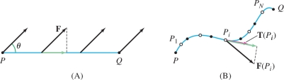
When the force acts on the object along a curved path \({\mathcal{C}}\), it makes sense to define the work \(W\) performed as the line integral [Figure 16.20]: \begin{equation*} \boxed{W = \int_{{\mathcal{C}}} {\bf{F}}{\cdot}\,d{\bf{s}}}\tag{9} \end{equation*}
This is the work “performed by the field \({\bf{F}}\).” The idea is that we can divide \({\mathcal{C}}\) into a large number of short consecutive arcs \({\mathcal{C}}_1,\ldots,{\mathcal{C}}_N\), where \({\mathcal{C}}_i\) has length \(\Delta s_i\). The work \(W_i\) performed along \({\mathcal{C}}_i\) is approximately equal to the tangential component \({\bf{F}}(P_i) {\cdot} {\bf{T}}(P_i)\) times the length \(\Delta s_i\), where \(P_i\) is a sample point in \({\mathcal{C}}_i\). Thus we have \[ W = \sum_{i=1}^N W_i \approx \sum_{i=1}^N ({\bf{F}}(P_i) {\cdot} {\bf{T}}(P_i))\Delta s_i \]
The right-hand side approaches \(\int_{{\mathcal{C}}} {\bf{F}}{\cdot} d{\bf{s}}\) as the lengths \(\Delta s_i\) tend to zero.
REMINDER
Work has units of energy. The SI unit of force is the newton, and the unit of energy is the joule, defined as 1 newton-meter. The British unit is the foot-pound.
Often, we are interested in calculating the work required to move an object along a path in the presence of a force field \({\bf{F}}\) (such as an electrical or gravitational field). In this case, \({\bf{F}}\) acts on the object and we must work against the force field to move the object. The work required is the negative of the line integral in Eq. (9): \[ \textrm{Work performed against }{\bf{F}} = -\int_{{\mathcal{C}}} {\bf{F}}{\cdot} d{\bf{s}} \]
EXAMPLE 8 Calculating Work
Calculate the work performed moving a particle from \(P=(0,0,0)\) to \(Q=(4,8,1)\) along the path \[ {\bf{c}}(t)= (t^2, t^3, t)\,\,\textrm{(in meters)}\qquad \textrm{for}\,\, 1\le t\le 2 \] in the presence of a force field \({\bf{F}}=\left\langle x^2, -z, -yz^{-1}\right\rangle\) in newtons.
Solution We have \[ \begin{array}{rl} {\bf{F}}({\bf{c}}(t)) &= {\bf{F}}(t^2, t^3, t) = \left\langle t^4,-t,-t^2\right\rangle\\ {\bf{c}}'(t) &= \left\langle 2t, 3t^2, 1\right\rangle\\ {\bf{F}}({\bf{c}}(t)) {\cdot} {\bf{c}}'(t) &= \big\langle t^4,-t,-t^2\big\rangle{\cdot} \big\langle 2t, 3t^2, 1\big\rangle = 2t^5-3t^3-t^2 \end{array} \]
957
The work performed against the force field in joules is \[ W = -\int_{{\mathcal{C}}} {\bf{F}} {\cdot} d{\bf{s}} = -\int_1^2(2t^5-3t^3-t^2)\,dt = \frac{89}{12} \]
Line integrals are also used to compute the “flux across a plane curve,” defined as the integral of the normal component of a vector field, rather than the tangential component (Figure 16.21). Suppose that a plane curve \({\mathcal{C}}\) is parametrized by \({\bf{c}}(t)\) for \(a\le t\le b\), and let \[ {\bf{n}} = {\bf{n}}(t)=\left\langle y'(t),-x'(t)\right\rangle,\qquad {\bf{e}}_n(t) = \frac{{\bf{n}}(t)}{\left \| {{\bf{n}}(t)} \right \|} \]
These vectors are normal to \({\mathcal{C}}\) and point to the right as you follow the curve in the direction of \({\bf{c}}\). The flux across \({\mathcal{C}}\) is the integral of the normal component \({\bf{F}}{\cdot}{\bf{e}}_n\), obtained by integrating \({\bf{F}}({\bf{c}}(t))\cdot{\bf{n}}(t)\): \begin{equation*} \textrm{Flux across }{\mathcal{C}} = \int_{\mathcal{C}}\,({\bf{F}}{\cdot} {\bf{e}}_n)ds = \int_a^b {\bf{F}}({\bf{c}}(t)){\cdot} {\bf{n}}(t)\,dt\tag{10} \end{equation*}
If \({\bf{F}}\) is the velocity field of a fluid (modeled as a two-dimensional fluid), then the flux is the quantity of water flowing across the curve per unit time.
EXAMPLE 9 Flux across a Curve
Calculate the flux of the velocity vector field \({\bf{v}}=\left\langle 3+2y-y^2/3,0\right\rangle\) (in centimeters per second) across the quarter ellipse \({\bf{c}}(t) = \left\langle 3\cos t, 6\sin t\right\rangle\) for \(0\le t\le \frac{\pi}2\) (Figure 16.22).
Solution The vector field along the path is \[ {\bf{v}}({\bf{c}}(t))=\left\langle 3+2(6\sin t)-(6\sin t)^2/3,0\right\rangle=\left\langle 3+12\sin t-12\sin^2 t,0\right\rangle \]
The tangent vector is \({\bf{c}}'(t)=\left\langle -3\sin t, 6\cos t\right\rangle\), and thus \({\bf{n}}(t)=\left\langle 6\cos t,3\sin t,\right\rangle\). We integrate the dot product \[ \begin{array}{rl} {\bf{v}}({\bf{c}}(t)){\cdot} {\bf{n}}(t) &= \left\langle 3+12\sin t-12\sin^2 t,0\right\rangle{\cdot}\left\langle 6\cos t,3\sin t,\right\rangle\\ &= (3+12\sin t-12\sin^2t)(6\cos t)\\ & = 18\cos t+72\sin t\cos t -72\sin^2t\cos t \end{array} \] to obtain the flux: \[ \begin{array}{rl} \int_a^b {\bf{v}}({\bf{c}}(t)){\cdot} {\bf{n}}(t)\,dt &=\int_0^{\pi/2}(18\cos t+72\sin t\cos t -72\sin^2t\cos t)\,dt\\ & = 18 + 36 -24 = 30\,\,\textrm{cm}^2\textrm{/s} \end{array} \]
16.2.1 Summary
- Line integral over a curve with parametrization \({\bf{c}}(t)\) for \(a\le t\le b\): \begin{array}{llll} &\textrm{Scalar line integral:}&\qquad &\int_{\mathcal{C}} f(x,y,z)\,ds = \int_a^b f({\bf{c}}(t))\,\left \| {{\bf{c}}'(t)} \right \|\,dt\\ &\textrm{Vector line integral:}&\qquad &\int_{\mathcal{C}} {\bf{F}}{\cdot} d{\bf{s}} = \int_{\mathcal{C}} ({\bf{F}}{\cdot}{\bf{T}})\,ds = \int_a^b {\bf{F}}({\bf{c}}(t)){\cdot}{\bf{c}}'(t)\,dt \end{array}
- Arc length differential: \(ds =\left \| {{\bf{c}}'(t)} \right \|\,dt\). To evaluate a scalar line integral, replace \(f(x,y,z)\,ds\) with \(f({\bf{c}}(t))\,\left \| {{\bf{c}}'(t)} \right \|\,dt\).
- Vector differential: \(d{\bf{s}} = {\bf{c}}'(t) \,dt\). To evaluate a vector line integral, replace \({\bf{F}}{\cdot}\,ds\) with \(F({\bf{c}}(t))\,{\cdot} {\bf{c}}'(t)\,dt\).
- An oriented curve \({\mathcal{C}}\) is a curve in which one of the two possible directions along \({\mathcal{C}}\) (called the positive direction) is chosen.
- The vector line integral depends on the orientation of the curve \({\mathcal{C}}\). The parametrization \({\bf{c}}(t)\) must be regular, and it must trace \({\mathcal{C}}\) in the positive direction.
- We write \(-{\mathcal{C}}\) for the curve \({\mathcal{C}}\) with the opposite orientation. Then \[ \int_{-{\mathcal{C}}} {\bf{F}}{\cdot} d{\bf{s}} = -\int_{{\mathcal{C}}} {\bf{F}}{\cdot} d{\bf{s}} \]
- If \(\rho(x,y,z)\) is the mass or charge density along \({\mathcal{C}}\), then the total mass or charge is equal to the scalar line integral \(\int_{\mathcal{C}} \rho(x,y,z)\,ds\).
- The vector line integral is used to compute the work \(W\) exerted on an object along a curve \({\mathcal{C}}\): \[ {W = \int_{\mathcal{C}}{\bf{F}}{\cdot} d{\bf{s}}} \] The work performed against \({\bf{F}}\) is the quantity \(-\int_{\mathcal{C}}{\bf{F}}{\cdot} d{\bf{s}}\).
958