16.3 Conservative Vector Fields
963
In this section we study conservative vector fields in greater depth. For convenience, when a particular parametrization \({\bf{c}}(t)\) of an oriented curve \({\mathcal{C}}\) is specified, we will denote the line integral \(\int_{\mathcal{C}} {\bf{F}} {\cdot} d{\bf{s}}\) by \[ \int_{\bf{c}}\,{\bf{F}}{\cdot}\,d{\bf{s}} \]
REMINDER
- A vector field \({\bf{F}}\) is conservative if \({\bf{F}} = \nabla V\) for some function \(V(x,y,z)\).
- \(V\) is called a potential function.
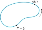
When the curve \({\mathcal{C}}\) is closed, we often refer to the line integral as the circulation of \({\bf{F}}\) around \({\mathcal{C}}\) (Figure 16.23) and denote it with the symbol \(\oint\): \[ \oint_{\mathcal{C}} {\bf{F}} {\cdot} d{\bf{s}} \]
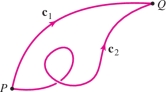
Our first result establishes the fundamental path independence of conservative vector fields, which means that the line integral of \({\bf{F}}\) along a path from \(P\) to \(Q\) depends only on the endpoints \(P\) and \(Q\), not on the particular path followed (Figure 16.24).
THEOREM 1 Fundamental Theorem for Conservative Vector Fields
Assume that \({\bf{F}}=\nabla{V}\) on a domain \({\mathcal{D}}\).
- 1. If \({\bf{c}}\) is a path from \(P\) to \(Q\) in \({\mathcal{D}}\), then \begin{equation*} \boxed{\int_{\bf{c}} {\bf{F}}{\cdot}\,d{\bf{s}} = {V}(Q)-{V}(P)}\tag{1} \end{equation*} In particular, \({\bf{F}}\) is path-independent.
- 2. The circulation around a closed path \({\bf{c}}\) (that is, \(P=Q\)) is zero: \[ \boxed{\oint_{\bf{c}}\,{\bf{F}}{\cdot} d{\bf{s}} = 0} \]
Proof Let \({\bf{c}}(t)\) be a path in \({\mathcal{D}}\) for \(a\le t\le b\) with \({\bf{c}}(a) = P\) and \({\bf{c}}(b)=Q\). Then \[ \int_{{\bf{c}}} {\bf{F}}{\cdot} d{\bf{s}} = \int_{{\bf{c}}} \nabla{V}{\cdot} d{\bf{s}} = \int_a^b \nabla{V}({\bf{c}}(t)){\cdot}{\bf{c}}'(t)\,dt \]
However, by the Chain Rule for Paths (Theorem 2 in Section 14.5), \[ \frac{d }{d t}{V}({\bf{c}}(t)) = \nabla {V}({\bf{c}}(t)){\cdot} {\bf{c}}'(t) \]
Thus we can apply the Fundamental Theorem of Calculus: \[ \int_{{\bf{c}}} {\bf{F}}{\cdot} d{\bf{s}} =\int_a^b \frac{d }{d t}{V}({\bf{c}}(t))\,dt = {V}({\bf{c}}(t))\Big|_a^b = {V}({\bf{c}}(b)) - {V}({\bf{c}}(a)) = {V}(Q)-{V}(P) \]
This proves Eq. (1). It also proves path independence, because the quantity \({V}(Q)-{V}(P)\) depends on the endpoints but not on the path \({\bf{c}}\). If \({\bf{c}}\) is a closed path, then \(P=Q\) and \({V}(Q)-{V}(P)=0\).
964
EXAMPLE 1
Let \({\bf{F}}=\left\langle 2xy+z,x^2,x \right\rangle\).
- (a) Verify that \({V}(x,y,z)=x^2y+xz\) is a potential function.
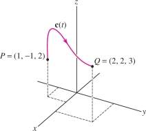
- (b) Evaluate \(\int_{\bf{c}}\,{\bf{F}}{\cdot}\,d{\bf{s}}\), where \({\bf{c}}\) is a path from \(P=(1,-1,2)\) to \(Q=(2, 2, 3)\).
Solution (a) The partial derivatives of \({V}(x,y,z) = x^2 y +xz\) are the components of \({\bf{F}}\): \[ \frac{\partial {V}}{\partial x} = 2xy+z,\qquad \frac{\partial {V}}{\partial y} = x^2,\qquad \frac{\partial {V}}{\partial z} = x \]
Therefore, \(\nabla{V} =\left\langle 2xy+z, x^2, x \right\rangle = {\bf{F}}\). (b) By Theorem 1, the line integral over any path \({\bf{c}}(t)\) from \(P = (1,-1,2)\) to \(Q=(2, 2, 3)\) [Figure 16.25] has the value \[ \begin{array}{rl} \int_{\bf{c}} {\bf{F}}{\cdot} d{\bf{s}}& = {V}(Q) - {V}(P)\\ & = {V}(2,2, 3) - {V}(1,-1,2)\\ & = \Big(2^2(2)+2(3)\Big) - \Big(1^2(-1)+1(2)\Big) = 13 \end{array} \]
EXAMPLE 2
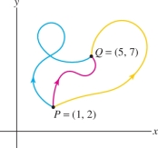
Find a potential function for \({\bf{F}}=\left\langle 2x+y,x \right\rangle\) and use it to evaluate \(\int_{\bf{c}} {\bf{F}}{\cdot} d{\bf{s}}\), where \({\bf{c}}\) is any path (Figure 16.26) from \((1,2)\) to \((5,7)\).
Solution We will develop a general method for finding potential functions. At this point we can see by inspection that \({V}(x,y) = x^2 + xy\) satisfies \(\nabla {V} = {\bf{F}}\): \[ \begin{array}{rl} \frac{\partial {V}}{\partial x} &= \frac{\partial }{\partial x} (x^2 + xy) = 2x + y,\\ \frac{\partial {V}}{\partial y} &= \frac{\partial }{\partial y}(x^2 + xy) = x \end{array} \]
Therefore, for any path \({\bf{c}}\) from \((1,2)\) to \((5,7)\), \[ \begin{array}{rl} \int_{\bf{c}} {\bf{F}} {\cdot} d{\bf{s}} &= {V}(5,7) - {V}(1,2)\\ & = (5^2 + 5(7)) - (1^2 + 1(2)) = 57 \end{array} \]
EXAMPLE 3 Integral around a Closed Path
Let \({V}(x,y,z)=xy\sin(yz)\). Evaluate \(\oint_{\mathcal{C}} \nabla{V}{\cdot} d{\bf{s}}\), where \({\mathcal{C}}\) is the closed curve in Figure 16.27.
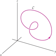
Solution By Theorem 1, the integral of a gradient vector around any closed path is zero. In other words, \(\oint_{\mathcal{C}} \nabla{V}{\cdot} d{\bf{s}} = 0\).
965
CONCEPTUAL INSIGHT
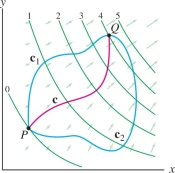
A good way to think about path independence is in terms of the contour map of the potential function. Consider a vector field \({\bf{F}}=\nabla{V}\) in the plane (Figure 16.28). The level curves of \({V}\) are called equipotential curves, and the value \(V(P)\) is called the potential at \(P\).
When we integrate \({\bf{F}}\) along a path \({\bf{c}}(t)\) from \(P\) to \(Q\), the integrand is \[ {\bf{F}}({\bf{c}}(t)){\cdot}{\bf{c}}'(t) = \nabla{V}({\bf{c}}(t)){\cdot}{\bf{c}}'(t) \]
Now recall that by the Chain Rule for paths, \[ \nabla{V}({\bf{c}}(t)){\cdot}{\bf{c}}'(t)) = \frac{d }{d t}{V}({\bf{c}}(t)) \]
In other words, the integrand is the rate at which the potential changes along the path, and thus the integral itself is the net change in potential: \[ \int {\bf{F}}{\cdot}\,d{\bf{s}} = \underbrace{V(Q)-V(P)}_{\textrm{Net change in potential}} \]
So informally speaking, what the line integral does is count the net number of equipotential curves crossed as you move along any path \(P\) to \(Q\). By “net number” we mean that crossings in the opposite direction are counted with a minus sign. This net number is independent of the particular path.
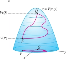
We can also interpret the line integral in terms of the graph of the potential function \(z={V}(x,y)\). The line integral computes the change in height as we move up the surface (Figure 16.29). Again, this change in height does not depend on the path from \(P\) to \(Q\). Of course, these interpretations apply only to conservative vector fields—otherwise, there is no potential function.
You might wonder whether there exist any path-independent vector fields other than the conservative ones. The answer is no. By the next theorem, a path-independent vector field is necessarily conservative.
THEOREM 1
A vector field \({\bf{F}}\) on an open connected domain \({\mathcal{D}}\) is path-independent if and only if it is conservative.
Proof We have already shown that conservative vector fields are path-independent. So we assume that \({\bf{F}}\) is path-independent and prove that \({\bf{F}}\) has a potential function.
To simplify the notation, we treat the case of a planar vector field \({\bf{F}}=\left\langle F_1, F_2\right\rangle\). The proof for vector fields in \({\bf{R}}^3\) is similar. Choose a point \(P_0\) in \({\mathcal{D}}\), and for any point \(P=(x,y)\in{\mathcal{D}}\), define \[ {V}(P)={V}(x,y)=\int_{{\bf{c}}} {\bf{F}}{\cdot} d{\bf{s}} \] where \({\bf{c}}\) is any path in \({\mathcal{D}}\) from \(P_0\) to \(P\) (Figure 16.30). Note that this definition of \({V}(P)\) is meaningful only because we are assuming that the line integral does not depend on the path \({\bf{c}}\).
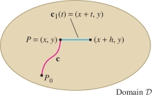
We will prove that \({\bf{F}}=\nabla V\), which involves showing that \(\frac{\partial {V}}{\partial x}=F_1\) and \(\frac{\partial {V}}{\partial y}=F_2\). We will only verify the first equation, as the second can be checked in a similar manner. Let \({\bf{c}}_1\) be the horizontal path \({\bf{c}}_1(t)=(x+t,y)\) for \(0\le t \le h\). For \(|h|\) small enough, \({\bf{c}}_1\) lies inside \({\mathcal{D}}\). Let \({\bf{c}}+{\bf{c}}_1\) denote the path \({\bf{c}}\) followed by \({\bf{c}}_1\). It begins at \(P_0\) and ends at \((x+h,y)\), so \[ \begin{array}{rl} {V}(x+h,y)-{V}(x,y) &= \int_{{\bf{c}}+{\bf{c}}_1}{\bf{F}}{\cdot} d{\bf{s}} - \int_{{\bf{c}}}{\bf{F}}{\cdot} d{\bf{s}} \\ & \left(\int_{{\bf{c}}} {\bf{F}}{\cdot} d{\bf{s}} + \int_{{\bf{c}}_1}{\bf{F}}{\cdot} d{\bf{s}}\right) - \int_{{\bf{c}}} {\bf{F}}{\cdot} d{\bf{s}} = \int_{{\bf{c}}_1} {\bf{F}}{\cdot} d{\bf{s}} \end{array} \]
966
The path \({\bf{c}}_1\) has tangent vector \({\bf{c}}_1'(t)=\left\langle 1,0 \right\rangle\), so \[ \begin{array}{rl} {\bf{F}}({\bf{c}}_1(t)){\cdot}{\bf{c}}_1'(t) &= \left\langle F_1(x+t,y),F_2(x+t,y) \right\rangle {\cdot} \left\langle 1,0 \right\rangle = F_1(x+t,y) \\ {V}(x+h,y)-{V}(x,y) &= \int_{{\bf{c}}_1} {\bf{F}} {\cdot} d{\bf{s}} = \int_0^h F_1(x+t,y)\,dt \end{array} \]
Using the substitution \(u=x+t\), we have \[ \frac{{V}(x+h,y)-{V}(x,y)}h = \frac1h \int_0^h F_1(x+t,y)\,dt = \frac1h \int_x^{x+h} F_1(u,y)\,du \]
The integral on the right is the average value of \(F_1(u,y)\) over the interval \([x,x+h]\). It converges to the value \(F_1(x,y)\) as \(h\to 0\), and this yields the desired result: \[ \frac{\partial {V}}{\partial x} = \lim_{h\to 0} \frac{{V}(x+h,y)-{V}(x,y)}h = \lim_{h\to 0} \frac1h \int_x^{x+h} F_1(u,y)\,du = F_1(x,y) \]
Conservative Fields in Physics
The Conservation of Energy principle says that the sum \(KE +PE\) of kinetic and potential energy remains constant in an isolated system. For example, a falling object picks up kinetic energy as it falls to earth, but this gain in kinetic energy is offset by a loss in gravitational potential energy (\(g\) times the change in height), such that the sum \(KE+PE\) remains unchanged.
We show now that conservation of energy is valid for the motion of a particle of mass \(m\) under a force field \({\bf{F}}\) if \({\bf{F}}\) has a potential function. This explains why the term “conservative” is used to describe vector fields that have a potential function. We follow the convention in physics of writing the potential function with a minus sign: \[ {\bf{F}} = -\nabla {V} \]
When the particle is located at \(P=(x,y,z)\), it is said to have potential energy \(V(P)\). Suppose that the particle moves along a path \({\bf{c}}(t)\). The particle’s velocity is \({\bf{v}} = {\bf{c}}'(t)\), and its kinetic energy is \(KE = \frac12m\left \| {\bf{v}} \right \|^2 = \frac12m{\bf{v}}{\cdot}{\bf{v}}\). By definition, the total energy at time \(t\) is the sum \[ E = KE + PE = \frac12m{\bf{v}}{\cdot}{\bf{v}} + {V}({\bf{c}}(t)) \]
In a conservative force field, the work \(W\) against \({\bf{F}}\) required to move the particle from \(P\) to \(Q\) is equal to the change in potential energy: \[ \begin{array}{rl} W &= -\int_{\bf{c}} \,{\bf{F}}{\cdot} d{\bf{s}} = {V}(Q)-{V}(P) \end{array} \]
THEOREM 3 Conservation of Energy
The total energy \(E\) of a particle moving under the influence of a conservative force field \({\bf{F}}=-\nabla V\) is constant in time. That is, \(\frac{d E}{d t}=0\).
967
Proof Let \({\bf{a}} = {\bf{v}}'(t)\) be the particle’s acceleration and let \(m\) be its mass. According to Newton’s Second Law of Motion, \({\bf{F}}({\bf{c}}(t))=m{\bf{a}}(t)\), and thus \[ \begin{array}{llll} \frac{d E}{d t} &=\frac{d }{d t}\left(\frac12m{\bf{v}}{\cdot}{\bf{v}} + {V}({\bf{c}}(t))\right)&&\\ &= m{\bf{v}}{\cdot}{\bf{a}} + \nabla{V}({\bf{c}}(t)){\cdot}{\bf{c}}'(t)&\qquad&\textrm{(Product and Chain Rules)}\\ &= {\bf{v}}{\cdot} m{\bf{a}} - {\bf{F}}{\cdot}{\bf{v}}&\qquad&\textrm{(since }{\bf{F}}=-\nabla{V}\textrm{ and }{\bf{c}}'(t) = {\bf{v}})\\ &= {\bf{v}}{\cdot}(m{\bf{a}} - {\bf{F}})=0&\qquad&\textrm{(since }{\bf{F}}=m{\bf{a}}) \end{array} \]
In Example 6 of Section 16.1, we verified that inverse-square vector fields are conservative: \[ {\bf{F}} = k\frac{{\bf{e}}_r}{r^2} = - \nabla{V}\quad\textrm{with}\quad {V} = \frac{k}r \]
Potential functions first appeared in 1774 in the writings of Jean-Louis Lagrange (1736–1813). One of the greatest mathematicians of his time, Lagrange made fundamental contributions to physics, analysis, algebra, and number theory. He was born in Turin, Italy, to a family of French origin but spent most of his career first in Berlin and then in Paris. After the French Revolution, Lagrange was required to teach courses in elementary mathematics, but apparently he spoke above the heads of his audience. A contemporary wrote, “whatever this great man says deserves the highest degree of consideration, but he is too abstract for youth.”
Basic examples of inverse-square vector fields are the gravitational and electrostatic forces due to a point mass or charge. By convention, these fields have units of force per unit mass or unit charge. Thus, if \({\bf{F}}\) is a gravitational field, the force on a particle of mass \(m\) is \(m{\bf{F}}\) and its potential energy is \(m{V}\), where \({\bf{F}} = -\nabla{V}\).
EXAMPLE 4 Work against Gravity
Compute the work \(W\) against the earth’s gravitational field required to move a satellite of mass \(m=600\) kg along any path from an orbit of altitude \(2000\) km to an orbit of altitude \(4000\) km.
Example 6 of Section 16.1 showed that \[ \frac{{\bf{e}}_r}{r^2} = -\nabla\left(\frac1r\right) \]
The constant \(k\) is equal to \(GM_e\) where \(G \approx 6.67\cdot 10^{-11}\) m\(^3\) kg\(^{-1}\) s\(^{-2}\) and the mass of the earth is \(M_e \approx 5.98 \cdot 10^{24}\) kg: \[ k = GM_e \approx 4\cdot 10^{14}\,\,\,\textrm{m}^3\,\textrm{s}^{-2} \]
Solution The earth’s gravitational field is the inverse-square field \[ {\bf{F}} = -k\frac{{\bf{e}}_r}{r^2} = -\nabla {V},\qquad\quad {V} = -\frac{k}r \] where \(r\) is the distance from the center of the earth and \(k=4\cdot 10^{14}\) (see marginal note). The radius of the earth is approximately \(6.4 \cdot 10^6\) meters, so the satellite must be moved from \(r= 8.4\cdot 10^6\) meters to \(r = 10.4\cdot 10^6\) meters. The force on the satellite is \(m{\bf{F}}=600{\bf{F}}\), and the work \(W\) required to move the satellite along a path \({\bf{c}}\) is \[ \begin{array}{rl} W &= -\int_{\bf{c}}\,m{\bf{F}}{\cdot} d{\bf{s}} = 600\int_{\bf{c}}\nabla{V}{\cdot} d{\bf{s}}\\ & = -\frac{600k}{r}\bigg|_{8.4\cdot 10^6}^{10.4 \times 10^{6}}\\ & \approx - \frac{2.4\cdot 10^{17}}{10.4\cdot 10^6} + \frac{2.4\cdot 10^{17}}{8.4\cdot 10^6} \approx 5.5\cdot 10^9~\textrm{joules} \end{array} \]
EXAMPLE 5
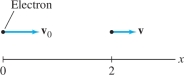
An electron is traveling in the positive \(x\)-direction with speed \(v_0 = 10^7\)~m/s. When it passes \(x = 0\), a horizontal electric field \({\bf{E}} = 100x {\bf{i}}\) (in newtons per coulomb) is turned on. Find the electron’s velocity after it has traveled 2 meters. Assume that \(q_e/m_e = -1.76 \cdot 10^{11}\)~C/kg, where \(q_e\) and \(m_e\) are the mass and charge of the electron, respectively.
Solution We have \({\bf{E}} = -\nabla V\) where \(V (x, y, z) = -50x^2\), so the electric field is conservative. Since \(V\) depends only on \(x\), we write \(V (x)\) for \(V (x, y, z)\). By the Law of Conservation of Energy, the electron’s total energy E is constant and therefore \(E\) has the same value when the electron is at \(x = 0\) and at \(x = 2\): \[ E =\frac{1}{2} m_e v^2_0 + q_e V (0) = \frac{1}{2} m_e v^2 + q_e V (2) \]
968
Since \(V (0) = 0\), we obtain \[ \frac{1}{2} m_e v^2_0 = \frac{1}{2} m_e v^2 + q_e V (2)\quad \Rightarrow\quad v = \sqrt{v^2_0 - 2(q_e/m_e)V (2)} \]
Using the numerical value of \(q_e/m_e\), we obtain \[ v \approx \sqrt{10^{14} - 2(-1.76 \cdot 10^{11})(-50(2)^2)}\approx\sqrt{2.96 \cdot 10^{13}} \approx 5.4 \cdot 10^6~\text{m/s} \]
Note that the velocity has decreased. This is because E exerts a force in the negative \(x\)-direction on a negative charge.
Finding Potential Functions
We do not yet have an effective way of telling whether a given vector field is conservative. By Theorem 1 in Section 16.1, every conservative vector field satisfies the cross-partials condition: \begin{equation*} \boxed{\frac{\partial F_1}{\partial y} = \frac{\partial F_2}{\partial x},\qquad \frac{\partial F_2}{\partial z} =\frac{\partial F_3}{\partial y},\qquad\frac{\partial F_3}{\partial x} = \frac{\partial F_1}{\partial z}}\tag{2} \end{equation*}
But does this condition guarantee that \({\bf{F}}\) is conservative? The answer is a qualified yes; the cross-partials condition does guarantee that \({\bf{F}}\) is conservative, but only on domains \({\mathcal{D}}\) with a property called simple-connectedness.
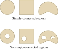
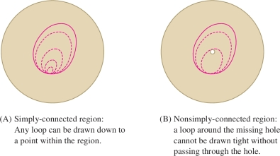
Roughly speaking, a domain \({\mathcal{D}}\) in the plane is simply-connected if it does not have any “holes” (Figure 16.32). More precisely, \({\mathcal{D}}\) is simply-connected if every loop in \({\mathcal{D}}\) can be drawn down, or “contracted,” to a point while staying within \({\mathcal{D}}\) as in Figure 16.33. Examples of simply-connected regions in \({\bf{R}}^2\) are disks, rectangles, and the entire plane \({\bf{R}}^2\). By contrast, the disk with a point removed in Figure 16.33 is not simply-connected: The loop cannot be drawn down to a point without passing through the point that was removed. In \({\bf{R}}^3\), the interiors of balls and boxes are simply-connected, as is the entire space \({\bf{R}}^3\).
THEOREM 4 Existence of a Potential Function
Let \({\bf{F}}\) be a vector field on a simply-connected domain \({\mathcal{D}}\). If \({\bf{F}}\) satisfies the cross-partials condition (2), then \({\bf{F}}\) is conservative.
969
Rather than prove Theorem 4, we illustrate a practical procedure for finding a potential function when the cross-partials condition is satisfied. The proof itself involves Stokes' Theorem and is somewhat technical because of the role played by the simply-connected property of the domain.
EXAMPLE 6 Finding a Potential Function
Show that \[ {\bf{F}} = \big\langle 2xy+y^3 , x^2+3xy^2+2y\big\rangle \] is conservative and find a potential function.
Solution First we observe that the cross-partial derivatives are equal: \[ \begin{array}{llll} \frac{\partial F_1}{\partial y} &= \frac{\partial}{\partial y}(2xy+y^3)& & = 2x+3y^2\\ \frac{\partial F_2}{\partial x} &= \frac{\partial}{\partial x} (x^2+3xy^2+2y)& &= 2x+3y^2 \end{array} \]
Furthermore, \({\bf{F}}\) is defined on all of \({\bf{R}}^2\), which is a simply-connected domain. Therefore, a potential function exists by Theorem 4.
Now, the potential function \(V\) satisfies \[ \frac{\partial {V}}{\partial x} = F_1(x,y) = 2xy+y^3 \]
This tells us that \({V}\) is an antiderivative of \(F_1(x,y)\), regarded as a function of \(x\) alone: \[ \begin{array}{rl} {V}(x,y) &= \int F_1(x,y)\, dx\\ & = \int \big(2xy+y^3\big)\, dx \\ & = x^2y + xy^3+ g(y) \end{array} \]
Note that to obtain the general antiderivative of \(F_1(x,y)\) with respect to \(x\), we must add on an arbitrary function \(g(y)\) depending on \(y\) alone, rather than the usual constant of integration. Similarly, we have \[ \begin{array}{rl} {V}(x,y) &= \int F_2(x,y)\, dy\\ & = \int \big(x^2+3xy^2+2y\big)\,dy\\ &= x^2y + xy^3 + y^2 + h(x) \end{array} \]
The two expressions for \({V}(x,y)\) must be equal: \[ x^2y + xy^3+ g(y) = x^2y+xy^3+y^2 + h(x) \]
This tells us that \(g(y)=y^2\) and \(h(x) = 0\), up to the addition of an arbitrary numerical constant \(C\). Thus we obtain the general potential function \[ {V}(x,y) = x^2y + xy^3+ y^2+C \]
The same method works for vector fields in three-space.
970
EXAMPLE 7
Find a potential function for \[ {\bf{F}} = \left\langle 2xyz^{-1} , z+x^2z^{-1} , y-x^2yz^{-2} \right\rangle \]
Solution If a potential function \(V\) exists, then it satisfies \[ \begin{array}{llll} V(x,y,z)&=\int 2xyz^{-1}\,dx &\;=\;& x^2yz^{-1}+f(y,z)\\ V(x,y,z)&=\int \big(z+x^2z^{-1}\big)\,dy &\;=\;& zy+x^2z^{-1}y+g(x,z)\\ V(x,y,z)&=\int \big(y-x^2yz^{-2}\big)\,dz &\;=\;& yz+x^2yz^{-1}+h(x,y) \end{array} \]
These three ways of writing \(V(x,y,z)\) must be equal: \[ x^2yz^{-1}+f(y,z) = zy+x^2z^{-1}y+g(x,z) = yz+x^2yz^{-1}+h(x,y) \]
These equalities hold if \(f(y,z)=yz\), \(g(x,z)=0\), and \(h(x,y)=0\). Thus \({\bf{F}}\) is conservative and, for any constant \(C\), a potential function is \[ V(x,y,z) = x^2yz^{-1} + yz +C \]
In Example 7, \({\bf{F}}\) is only defined for \(z\ne 0\), so the domain has two halves: \(z>0\) and \(z<0\). We are free to choose different constants \(C\) on the two halves, if desired.
Assumptions Matter We cannot expect the method for finding a potential function to work if \({\bf{F}}\) does not satisfy the cross-partials condition (because in this case, no potential function exists). What goes wrong? Consider \({\bf{F}}=\left\langle y,0\right\rangle\). If we attempted to find a potential function, we would calculate \[ \begin{array}{rl} {V}(x,y) &= \int y\,dx = xy+g(y)\\ {V}(x,y) &= \int 0\,dy = 0+h(x) \end{array} \]
However, there is no choice of \(g(y)\) and \(h(x)\) for which \(xy+g(y)=h(x)\). If there were, we could differentiate this equation twice, once with respect to \(x\) and once with respect to~\(y\). This would yield \(1 = 0\), which is a contradiction. The method fails in this case because \({\bf{F}}\) does not satisfy the cross-partials condition and thus is not conservative.
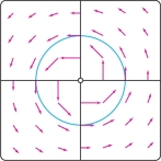
The Vortex Field Why does Theorem 4 assume that the domain is simply-connected? This is an interesting question that we can answer by examining the vortex field (Figure 16.34): \[ {\bf{F}} = \left\langle \frac{-y}{x^2+y^2}, \frac{x}{x^2+y^2}\right\rangle \]
EXAMPLE 8
Show that the vortex field satisfies the cross-partials condition but is not conservative. Does this contradict Theorem 4?
Solution We check the cross-partials condition directly: \[ \begin{array}{rl} \frac{\partial }{\partial x}\left(\frac{x}{x^2+y^2}\right) &=\frac{(x^2+y^2)-x(\partial/\partial x)(x^2+y^2)}{(x^2+y^2)^2}=\frac{y^2-x^2}{(x^2+y^2)^2}\\ \frac{\partial }{\partial y}\left(\frac{-y}{(x^2+y^2)}\right) &=\frac{-(x^2+y^2) + y(\partial/\partial y)(x^2+y^2)}{(x^2+y^2)^2}=\frac{y^2-x^2}{(x^2+y^2)^2} \end{array} \]
Now consider the line integral of \({\bf{F}}\) around the unit circle \({\mathcal{C}}\) parametrized by \({\bf{c}}(t)=(\cos t,\sin t)\): \begin{equation*} \begin{array}{rcl} F({\bf{c}}(t)){\cdot}{\bf{c}}'(t) &=& \left\langle -\sin t,\cos t\right\rangle{\cdot}\left\langle -\sin t,\cos t\right\rangle =\sin^2t+\cos^2t = 1\\ \oint_{\bf{c}} {\bf{F}}{\cdot} d{\bf{s}} &=& \int_0^{2\pi} {\bf{F}}({\bf{c}}(t)){\cdot}{\bf{c}}'(t)\,dt = \int_0^{2\pi} dt = 2\pi \ne 0 \end{array}\tag{3} \end{equation*}
971
If \({\bf{F}}\) were conservative, its circulation around every closed curve would be zero by Theorem 1. Thus \({\bf{F}}\) cannot be conservative, even though it satisfies the cross-partials condition.
This result does not contradict Theorem 4 because the domain of \({\bf{F}}\) does not satisfy the simply-connected condition of the theorem. Because \({\bf{F}}\) is not defined at \((x,y)=(0,0)\), its domain is \({\mathcal{D}}=\{(x,y)\ne (0,0)\}\), and this domain is not simply-connected (Figure 16.35).

CONCEPTUAL INSIGHT
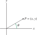
Although the vortex field \({\bf{F}}\) is not conservative on its domain, it is conservative on any smaller, simply-connected domain, such as the upper half-plane \(\{(x,y): y>0\}\). In fact, we can show (see the marginal note) that \({\bf{F}} = \nabla {V}\), where \[ {V}(x,y) = \theta =\tan^{-1}\frac{y}x \]
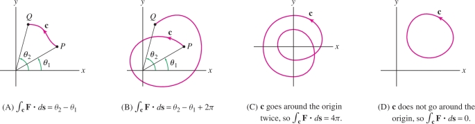
By definition, then, the potential \(V(x,y)\) at any point \((x,y)\) is the angle \(\theta\) of the point in polar coordinates (Figure 16.36). The line integral of \({\bf{F}}\) along a path \({\bf{c}}\) is equal to the change in potential \(\theta\) along the path Figure 16.37]: \[ \int_{\bf{c}} {\bf{F}}{\cdot} d{\bf{s}} = \theta_2-\theta_1 = \textrm{the change in angle }\theta\textrm{ along }{\bf{c}} \]
Now we can see what is preventing \({\bf{F}}\) from being conservative on all of its domain. The angle \(\theta\) is defined only up to integer multiples of \(2\pi\). The angle along a path that goes all the way around the origin does not return to its original value but rather increases by \(2\pi\). This explains why the line integral around the unit circle (Eq. 3) is \(2\pi\) rather than \(0\). And it shows that \(V(x,y) = \theta\) cannot be defined as a continuous function on the entire domain \({\mathcal{D}}\). However, \(\theta\) is continuous on any domain that does not enclose the origin, and on such domains we have \({\bf{F}}=\nabla\theta\).
In general, if a closed path \({\bf{c}}\) winds around the origin \(n\) times (where \(n\) is negative if the curve winds in the clockwise direction), then [Figures 15(C) and (D)]: \[ \oint_{\bf{c}} {\bf{F}}{\cdot} d{\bf{s}} = 2\pi n \]
The number \(n\) is called the winding number of the path. It plays an important role in the mathematical field of topology.
Using the Chain Rule and the formula \[ \frac{d }{d t}\tan^{-1}t=\frac1{1+t^2} \] we can check that \({\bf{F}} = \nabla V\) \[ \begin{array}{rl} \frac{\partial \theta}{\partial x} = \frac{\partial}{\partial x}\tan^{-1}\frac{y}x & = \frac{-y/x^2}{1+(y/x)^2} = \frac{-y}{x^2+y^2}\\ \frac{\partial \theta}{\partial y} = \frac{\partial}{\partial y}\tan^{-1} \frac{y}x & = \frac{1/x}{1+(y/x)^2} = \frac{x}{x^2+y^2} \end{array} \]
16.3.1 Summary
972
- A vector field \({\bf{F}}\) on a domain \({\mathcal{D}}\) is conservative if there exists a function \({V}\) such that \(\nabla{V}={\bf{F}}\) on \({\mathcal{D}}\). The function \({V}\) is called a potential function of \({\bf{F}}\).
- A vector field \({\bf{F}}\) on a domain \({\mathcal{D}}\) is called path-independent if for any two points \(P, Q\in {\mathcal{D}}\), we have \[ \int_{{\bf{c}}_1} {\bf{F}}{\cdot} d{\bf{s}} = \int_{{\bf{c}}_2} {\bf{F}}{\cdot} d{\bf{s}} \] for any two paths \({\bf{c}}_1\) and \({\bf{c}}_2\) in \({\mathcal{D}}\) from \(P\) to \(Q\).
- The Fundamental Theorem for Conservative Vector Fields: If \({\bf{F}}=\nabla{V}\), then \[ \int_{{\bf{c}}} {\bf{F}}{\cdot} d{\bf{s}} = {V}(Q)-{V}(P) \] for any path \({\bf{c}}\) from \(P\) to \(Q\) in the domain of \({\bf{F}}\). This shows that conservative vector fields are path-independent. In particular, if \({\bf{c}}\) is a closed path (\(P=Q\)), then \[ \oint_{{\bf{c}}} {\bf{F}}{\cdot} d{\bf{s}} = 0 \]
- The converse is also true: On an open, connected domain, a path-independent vector field is conservative.
- Conservative vector fields satisfy the cross-partial condition \begin{equation*} \frac{\partial F_1}{\partial y} = \frac{\partial F_2}{\partial x},\qquad \frac{\partial F_2}{\partial z} = \frac{\partial F_3}{\partial y},\qquad\frac{\partial F_3}{\partial x} = \frac{\partial F_1}{\partial z}\tag{4} \end{equation*}
- Equality of the cross-partials guarantees that \({\bf{F}}\) is conservative if the domain \({\mathcal{D}}\) is simply connected—that is, if any loop in \({\mathcal{D}}\) can be drawn down to a point within \({\mathcal{D}}\).