16.4 Parametrized Surfaces and Surface Integrals
The basic idea of an integral appears in several guises. So far, we have defined single, double, and triple integrals and, in the previous section, line integrals over curves. Now we consider one last type on integral: integrals over surfaces. We treat scalar surface integrals in this section and vector surface integrals in the following section.
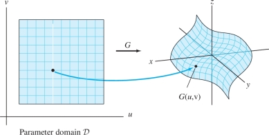
Just as parametrized curves are a key ingredient in the discussion of line integrals, surface integrals require the notion of a parametrized surface—that is, a surface \({\mathcal{S}}\) whose points are described in the form \[ {G}(u,v) = (x(u,v), y(u,v), z(u,v)) \]
The variables \(u, v\) (called parameters) vary in a region \({\mathcal{D}}\) called the parameter domain. Two parameters \(u\) and \(v\) are needed to parametrize a surface because the surface is two-dimensional. Figure 16.38 shows a plot of the surface \({\mathcal{S}}\) with the parametrization \[ {G}(u,v) = (u + v, u^3 - v, v^3 - u) \]
975
This surface consists of all points \((x,y,z)\) in \({\bf{R}}^3\) such that \[ x = u+v,\qquad y = u^3 -v,\qquad z = v^3-u \] for \((u,v)\) in \({\mathcal{D}} = {\bf{R}}^2\).
EXAMPLE 1 Parametrization of a Cone
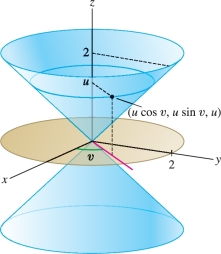
Find a parametrization of the portion \({\mathcal{S}}\) of the cone with equation \(x^2+y^2=z^2\) lying above or below the disk \(x^2+y^2\le 4\). Specify the domain \({\mathcal{D}}\) of the parametrization.
Solution This surface \(x^2+y^2=z^2\) is a cone whose horizonal cross section at height \(z=u\) is the circle \(x^2+y^2=u^2\) of radius \(u\) (Figure 16.39). So a point on the cone at height \(u\) has coordinates \((u\cos v, u\sin v, u)\) for some angle \(v\). Thus, the cone has the parametrization \[ {G}(u,v) = (u\cos v, u\sin v, u) \]
Since we are interested in the portion of the cone where \(x^2+y^2=u^2\le 4\), the height variable \(u\) satisfies \(-2\le u \le 2\). The angular variable \(v\) varies in the interval \([0,2\pi)\), and therefore, the parameter domain is \({\mathcal{D}} = [-2,2]\times[0,2\pi)\).
If necessary, review cylindrical and spherical coordinates in Section 12.7. They are used often in surface calculations.
Three standard parametrizations arise often in computations. First, the cylinder of radius \(R\) with equation \(x^2+y^2=R^2\) is conveniently parametrized in cylindrical coordinates (Figure 16.40). Points on the cylinder have cylindrical coordinates \((R,\theta,z)\), so we use \(\theta\) and \(z\) as parameters (with fixed \(R\)).
Parametrization of a Cylinder:
\[ \boxed{{G}(\theta,z) = (R\cos\theta,R\sin\theta,z),\qquad 0\le \theta<2\pi,\quad -\infty< z<\infty } \]

976
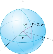
The sphere of radius \(R\) with center at the origin is parametrized conveniently using spherical coordinates \((\rho,\theta,\phi)\) with \(\rho=R\) (Figure 16.41).
Parametrization of a Sphere:
\[ \boxed{{G}(\theta,\phi) = (R\cos\theta\sin\phi,R\sin\theta\sin\phi, R\cos\phi),\quad 0\le \theta < 2\pi,\quad 0\le \phi\le\pi} \]
The North and South Poles correspond to \(\phi = 0\) and \(\phi=\pi\) with any value of \(\theta\) (the map \({G}\) fails to be one-to-one at the poles): \[ \textrm{North Pole:}~ {G}(\theta,0)=(0,0,R),\qquad \textrm{South Pole:}~{G}(\theta,\pi)=(0,0,-R) \]
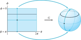
As shown in Figure 16.42, \({G}\) maps each horizontal segment \(\phi=c\) (\(0<c<\pi\)) to a latitude (a circle parallel to the equator) and each vertical segment \(\theta=c\) to a longitudinal arc from the the North Pole to the South Pole.
Finally, the graph of a function \(z=f(x,y)\) always has the following simple parametrization (Figure 16.43).
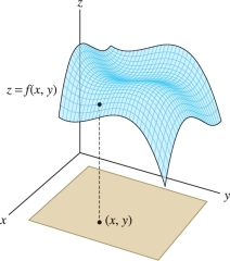
Parametrization of a Graph:
\[ \boxed{{G}(x,y)=(x,y,f(x,y))} \]
In this case, the parameters are \(x\) and \(y\).
Grid Curves, Normal Vectors, and the Tangent Plane
Suppose that a surface \({\mathcal{S}}\) has a parametrization \[ {G}(u,v) = (x(u,v), y(u,v), z(u,v)) \] that is one-to-one on a domain \({\mathcal{D}}\). We shall always assume that \({G}\) is continuously differentiable, meaning that the functions \(x(u,v)\), \(y(u,v)\), and \(z(u,v)\) have continuous partial derivatives.
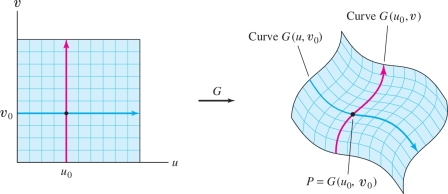
In essence, a parametrization labels each point \(P\) on \({\mathcal{S}}\) by a unique pair \((u_0,v_0)\) in the parameter domain. We can think of \((u_0,v_0)\) as the “coordinates” of \(P\) determined by the parametrization. They are sometimes called curvilinear coordinates.
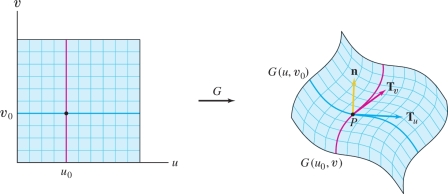
In the \(uv\)-plane, we can form a grid of lines parallel to the coordinates axes. These grid lines correspond under \({G}\) to a system of grid curves on the surface (Figure 16.44). More precisely, the horizontal and vertical lines through \((u_0,v_0)\) in the domain correspond to the grid curves \({G}(u,v_0)\) and \({G}(u_0,v)\) that intersect at the point \(P={G}(u_0,v_0)\).
977
Now consider the tangent vectors to these grid curves (Figure 16.45): \[ \begin{array}{llll} &\textrm{For }G(u,v_0):&\quad{\bf{T}}_u(P) &= \frac{\partial {G}}{\partial u}(u_0,v_0) = \left\langle \frac{\partial x}{\partial u}(u_0,v_0) ,\frac{\partial y}{\partial u}(u_0,v_0) ,\frac{\partial z}{\partial u}(u_0,v_0) \right\rangle\\ &\textrm{For }G(u_0,v):&\quad{\bf{T}}_v(P) &= \frac{\partial {G}}{\partial v}(u_0,v_0) = \left\langle \frac{\partial x}{\partial v}(u_0,v_0) ,\frac{\partial y}{\partial v}(u_0,v_0) ,\frac{\partial z}{\partial v}(u_0,v_0) \right\rangle \end{array} \]
The parametrization \({G}\) is called regular at \(P\) if the following cross product is nonzero: \[ {\bf{n}}(P) = {\bf{n}}(u_0,v_0)= {\bf{T}}_u(P){\times}{\bf{T}}_v(P) \]
In this case, \({\bf{T}}_u\) and \({\bf{T}}_v\) span the tangent plane to \({\mathcal{S}}\) at \(P\) and \({\bf{n}}(P)\) is a normal vector to the tangent plane. We call \({\bf{n}}(P)\) a normal to the surface \({\mathcal{S}}\).
At each point on a surface, the normal vector points in one of two opposite directions. If we change the parametrization, the length of \({\bf{n}}\) may change and its direction may be reversed.
We often write \({\bf{n}}\) instead of \({\bf{n}}(P)\) or \({\bf{n}}(u,v)\), but it is understood that the vector \({\bf{n}}\) varies from point to point on the surface. Similarly, we often denote the tangent vectors by \({\bf{T}}_u\) and \({\bf{T}}_v\). Note that \({\bf{T}}_u\), \({\bf{T}}_v\), and \({\bf{n}}\) need not be unit vectors (thus the notation here differs from that in Sections 13.4, 13.5, and 16.2, where \({\bf{T}}\) and \({\bf{n}}\) denote unit vectors).
EXAMPLE 2
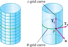
Consider the parametrization \({G}(\theta,z)=(2\cos\theta, 2\sin\theta, z)\) of the cylinder \(x^2+y^2=4\):
- (a) Describe the grid curves.
- (b) Compute \({\bf{T}}_\theta\), \({\bf{T}}_z\), and \({\bf{n}}(\theta,z)\).
- (c) Find an equation of the tangent plane at \(P={G}(\frac{\pi}4,5)\).
Solution
- (a) The grid curves on the cylinder through \(P = (\theta_0,z_0)\) are (Figure 16.46) \[ \begin{array}{llllll} &\theta\textrm{-grid curve:}\,\,\, &G(\theta,z_0)=&(2\cos\theta, 2\sin\theta, z_0)&\qquad &\textrm{(circle of radius 2 at height }z = z_0) \\ &z\textrm{-grid curve:}\,\,\, &G(\theta_0,z){}={}&(2\cos\theta_0, 2\sin\theta_0, z) & \qquad&\textrm{(vertical line through } P\textrm{ with } \theta=\theta_0) \end{array} \]
- (b) The partial derivatives of \({G}(\theta,z)=(2\cos\theta, 2\sin\theta, z)\) give us the tangent vectors at \(P\): \[ \begin{array}{llll} &\theta\textrm{-grid curve:}\quad &{\bf{T}}_\theta &= \frac{\partial {G}}{\partial \theta} = \frac{\partial }{\partial \theta}(2\cos\theta, 2\sin\theta, z)= \left\langle -2\sin \theta, 2\cos \theta,0 \right\rangle\\ &z\textrm{-grid curve:}\quad& {\bf{T}}_z &= \frac{\partial {G}}{\partial z} =\frac{\partial}{\partial z} (2\cos\theta, 2\sin\theta, z)= \left\langle 0, 0, 1\right\rangle \end{array} \] Observe in Figure 16.46 that \({\bf{T}}_\theta\) is tangent to the \(\theta\)-grid curve and \({\bf{T}}_z\) is tangent to the \(z\)-grid curve. The normal vector is \[ {\bf{n}}(\theta,z) = {\bf{T}}_\theta{\times}{\bf{T}}_z = \left| \begin{array}{ccc} {\bf{i}} & {\bf{j}} & {\bf{k}} \\ -2\sin\theta & 2\cos \theta & 0 \\ 0 & 0 & 1 \end{array} \right| = 2\cos \theta {\bf{i}} +2\sin\theta {\bf{j}} \] The coefficient of \({\bf{k}}\) is zero, so \({\bf{n}}\) points directly out of the cylinder.
- (c) For \(\theta=\frac{\pi}4\), \(z=5\), \[ P = {G}\left(\frac{\pi}4,5\right) = \big\langle\sqrt 2,\sqrt 2,5\big\rangle, \qquad {\bf{n}} = {\bf{n}}\left(\frac{\pi}4,5\right) =\big\langle\sqrt 2,\sqrt 2,0\big\rangle \] The tangent plane through \(P\) has normal vector \({\bf{n}}\) and thus has equation \[ \big\langle x-\sqrt 2, y-\sqrt 2, z-5\big\rangle{\cdot} \big\langle\sqrt 2,\sqrt 2,0\big\rangle = 0 \] This can be written \[ \sqrt 2(x-\sqrt 2)+ \sqrt 2(y-\sqrt 2) = 0\qquad\textrm{or}\qquad x+y=2\sqrt2 \] The tangent plane is vertical (because \(z\) does not appear in the equation).
978
REMINDER
An equation of the plane through \(P=(x_0,y_0,z_0)\) with normal vector \({\bf{n}}\) is \[ \big\langle x-x_0, y-y_0, z-z_0\big\rangle{\cdot} {\bf{n}} = 0 \]
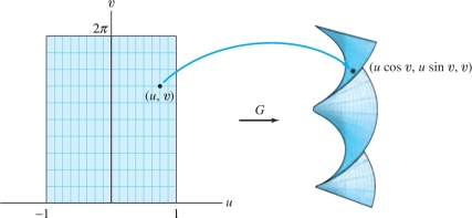
EXAMPLE 5 Helicoid Surface
![]() Describe the surface \({\mathcal{S}}\) with parametrization
\[
{G}(u,v) = (u\cos v, u\sin v, v),\qquad -1\le u\le 1,\quad 0\le v< 2\pi
\]
Describe the surface \({\mathcal{S}}\) with parametrization
\[
{G}(u,v) = (u\cos v, u\sin v, v),\qquad -1\le u\le 1,\quad 0\le v< 2\pi
\]
- (a) Use a computer algebra system to plot \({\mathcal{S}}\).
- (b) Compute \({\bf{n}}(u,v)\) at \(u=\frac12\), \(v=\frac{\pi}2\).
Solution For each fixed value \(u=a\), the curve \({G}(a,v)=(a\cos v, a\sin v, v)\) is a helix of radius \(a\). Therefore, as \(u\) varies from \(-1\) to \(1\), \({G}(u,v)\) describes a family of helices of radius \(u\). The resulting surface is a “helical ramp.”
(a) Here is a typical command for a computer algebra system that generates the helicoid surface shown on the right-hand side of Figure 16.47.
ParametricPlot3D[{u*Cos[v],u*Sin[v],v},{u,-1,1},{v,0,2Pi}]
- (b) The tangent and normal vectors are \[ \begin{array}{rl} {\bf{T}}_u &= \frac{\partial {G}}{\partial u} = \left\langle \cos v, \sin v,0 \right\rangle\\ {\bf{T}}_v &= \frac{\partial {G}}{\partial v} = \left\langle -u\sin v, u\cos v, 1\right\rangle\\ {\bf{n}}(u,v) &= {\bf{T}}_u{\times}{\bf{T}}_v = \left| \begin{array}{ccc} {\bf{i}} & {\bf{j}} & {\bf{k}} \\ \cos v & \sin v & 0 \\ -u\sin v & u\cos v & 1 \\ \end{array} \right|= (\sin v){\bf{i}} - (\cos v){\bf{j}} + u{\bf{k}} \end{array} \] At \(u = \frac12\), \(v = \frac{\pi}2\), we have \({\bf{n}} = {\bf{i}} +\tfrac12{\bf{k}}\).
979
For future reference, we compute the outward-pointing normal vector in the standard parametrization of the sphere of radius \(R\) centered at the origin (Figure 16.48): \[ {G}(\theta,\phi)=(R\cos\theta\sin\phi,R\sin\theta\sin\phi,R\cos\phi) \]
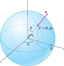
Note first that since the distance from \({G}(\theta,\phi)\) to the origin is \(R\), the unit radial vector at \({G}(\theta,\phi)\) is obtained by dividing by \(R\): \[ {\bf{e}}_r = \left\langle \cos\theta\sin\phi,\sin\theta\sin\phi,\cos\phi \right\rangle \]
Furthermore, \begin{equation*} \begin{array}{rl} {\bf{T}}_{\theta} &= \left\langle -R\sin\theta\sin\phi , R\cos\theta\sin\phi , 0\right\rangle\\ {\bf{T}}_{\phi} &=\left\langle R\cos\theta\cos\phi , R\sin\theta\cos\phi, -R\sin\phi\right\rangle \\ {\bf{n}} &= {\bf{T}}_{\theta}{\times}{\bf{T}}_{\phi} = \left| \begin{array}{ccc} {\bf{i}} & {\bf{j}} & {\bf{k}} \\ -R\sin\theta\sin\phi & R\cos\theta\sin\phi & 0\\ R\cos\theta\cos\phi & R\sin\theta\cos\phi & -R\sin\phi \\ \end{array} \right|\\ & = -R^2\cos\theta\sin^2\phi\,{\bf{i}} - R^2\sin\theta\sin^2\phi\,{\bf{j}} -R^2\cos\phi\sin\phi\,{\bf{k}}\\ & = -R^2\sin\phi\left\langle \cos\theta\sin\phi, \sin\theta\sin\phi, \cos\phi \right\rangle\\ &=-(R^2\sin \phi)\,{\bf{e}}_r \end{array}\tag{1} \end{equation*}
This is an inward-pointing normal vector. However, in most computations it is standard to use the outward-pointing normal vector: \begin{equation*} \boxed{{\bf{n}} = {\bf{T}}_{\phi} {\times} {\bf{T}}_{\theta} = (R^2\sin\phi)\,{\bf{e}}_r,\qquad \qquad \left \| {\bf{n}} \right \| = R^2\sin\phi}\tag{2} \end{equation*}
Surface Area
The length \(\left \| {\bf{n}} \right \|\) of the normal vector in a parametrization has an important interpretation in terms of area. Assume, for simplicity, that \({\mathcal{D}}\) is a rectangle (the argument also applies to more general domains). Divide \({\mathcal{D}}\) into a grid of small rectangles \({\mathcal{R}}_{ij}\) of size \(\Delta u\times\Delta v\), as in Figure 16.49, and compare the area of \({\mathcal{R}}_{ij}\) with the area of its image under \({G}\). This image is a “curved” parallelogram \({\mathcal{S}}_{ij} = {G}({\mathcal{R}}_{ij})\).
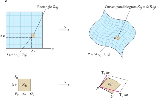
First, we note that if \(\Delta u\) and \(\Delta v\) in Figure 16.49 are small, then the curved parallelogram \({\mathcal{S}}_{ij}\) has approximately the same area as the “genuine” parallelogram with sides \(\overrightarrow{PQ}\) and \(\overrightarrow{PS}\). Recall that the area of the parallelogram spanned by two vectors is the length of their cross product, so \[ \textrm{Area}({\mathcal{S}}_{ij}) \approx \left \| {\overrightarrow{PQ}{\times}\overrightarrow{PS}} \right \| \]
980
REMINDER
By Theorem 3 in Section 12.4, the area of the parallelogram spanned by vectors \({\bf{v}}\) and \({\bf{w}}\) in \({\bf{R}}^3\) is equal to \(\left \| {{\bf{v}}{\times}{\bf{w}}} \right \|\).
Next, we use the linear approximation to estimate the vectors \(\overrightarrow{PQ}\) and \(\overrightarrow{PS}\): \[ \begin{array}{rl} \overrightarrow{PQ}={G}(u_{ij}+\Delta u,v_{ij})-{G}(u_{ij},v_{ij})&\approx \frac{\partial {G}}{\partial u}(u_{ij},v_{ij})\Delta u ={\bf{T}}_u\Delta u \\ \overrightarrow{PS}= {G}(u_{ij},v_{ij}+\Delta v)-{G}(u_{ij},v_{ij})&\approx \frac{\partial {G}}{\partial v}(u_{ij},v_{ij})\Delta v = {\bf{T}}_v\Delta v \end{array} \]
Thus we have \[ \textrm{Area}({\mathcal{S}}_{ij}))\approx \left \| {{\bf{T}}_u\Delta u{\times}{\bf{T}}_v\Delta v}\right \| = \left \| {{\bf{T}}_u{\times}{\bf{T}}_v} \right \|\,\Delta u\,\Delta v \]
Since \({\bf{n}}(u_{ij},v_{ij})={\bf{T}}_u{\times}{\bf{T}}_v\) and \(\mathrm{Area}({\mathcal{R}}_{ij})=\Delta u\Delta v\), we obtain \begin{equation*} \boxed{\textrm{Area}({\mathcal{S}}_{ij}) \approx \left \| {{\bf{n}}(u_{ij},v_{ij})} \right \|\textrm{Area}({\mathcal{R}}_{ij})}\tag{3} \end{equation*}
Our conclusion: \(\left \| {\bf{n}} \right \|\) is a distortion factor that measures how the area of a small rectangle \({\mathcal{R}}_{ij}\) is altered under the map \({G}\).
The approximation (3) is valid for any small region \({\mathcal{R}}\) in the \(uv\)-plane: \[ \mathrm{Area}({\mathcal{S}}) \approx \left \| {{\bf{n}}(u_0,v_0))} \right \|\mathrm{Area}({\mathcal{R}}) \] where \({\mathcal{S}}={G}({\mathcal{R}})\) and \((u_0,v_0)\) is any sample point in \({\mathcal{R}}\). Here, “small” means contained in a small disk. We do not allow \({\mathcal{R}}\) to be very thin and wide.
Note: We require only that \({G}\) be one-to-one on the interior of \({\mathcal{D}}\). Many common parametrizations (such as the parametrizations by cylindrical and spherical coordinates) fail to be one-to-one on the boundary of their domains.
To compute the surface area of \({\mathcal{S}}\), we assume that \({G}\) is one-to-one, except possibly on the boundary of \({\mathcal{D}}\). We also assume that \({G}\) is regular, except possibly on the boundary of \({\mathcal{D}}\). Recall that “regular” means that \({\bf{n}}(u,v)\) is nonzero.
The entire surface \({\mathcal{S}}\) is the union of the small patches \({\mathcal{S}}_{ij}\), so we can apply the approximation on each patch to obtain \begin{equation*} \textrm{Area}({\mathcal{S}}) = \sum_{i,j}\textrm{Area}({\mathcal{S}}_{ij}) \approx \sum_{i,j} \left \| {{\bf{n}}(u_{ij},v_{ij})} \right \|\Delta u\Delta v\tag{4} \end{equation*}
The sum on the right is a Riemann sum for the double integral of \(\left \| {{\bf{n}}(u,v)} \right \|\) over the parameter domain \({\mathcal{D}}\). As \(\Delta u\) and \(\Delta v\) tend to zero, these Riemann sums converge to a double integral, which we take as the definition of surface area: \[ \boxed{\textrm{Area}({\mathcal{S}}) = \iint_{{\mathcal{D}}\,} \left \| {{\bf{n}}(u,v)} \right \|\,du\,dv} \]
Surface Integral
981
Now we can define the surface integral of a function \(f(x,y,z)\): \[ \iint_{{\mathcal{S}}\,}\,f(x,y,z)\,dS \]
This is similar to the definition of the line integral of a function over a curve. Choose a sample point \(P_{ij} = {G}(u_{ij},v_{ij})\) in each small patch \({\mathcal{S}}_{ij}\) and form the sum: \begin{equation*} \sum_{i,j} f(P_{ij})\textrm{Area}({\mathcal{S}}_{ij})\tag{5} \end{equation*}
The limit of these sums as \(\Delta u\) and \(\Delta v\) tend to zero (if it exists) is the surface integral: \[ \iint_{{\mathcal{S}}\,}\,f(x,y,z)\,dS = \lim_{\Delta u, \Delta v\to 0} \sum_{i,j} f(P_{ij})\textrm{Area}({\mathcal{S}}_{ij}) \]
To evaluate the surface integral, we use Eq. (3) to write \begin{equation*} \sum_{i,j}f(P_{ij})\textrm{Area}({\mathcal{S}}_{ij}) \approx \sum_{i,j} f({G}(u_{ij},v_{ij})) \left \| {{\bf{n}}(u_{ij},v_{ij})} \right \|\,\Delta u\,\Delta v\tag{6} \end{equation*}
On the right we have a Riemann sum for the double integral of \[ f({G}(u,v))\left \| {{\bf{n}}(u,v)} \right \| \] over the parameter domain \({\mathcal{D}}\). Under the assumption that \({G}\) is continuously differentiable, we can show these the sums in Eq. (6) approach the same limit. This yields the next theorem.
It is interesting to note that Eq. (7) includes the Change of Variables Formula for double integrals (Theorem 1 in Section 15.6) as a special case. If the surface \({\mathcal{S}}\) is a domain in the \(xy\)-plane [in other words, \(z(u,v)=0\)], then the integral over \({\mathcal{S}}\) reduces to the double integral of the function \(f(x,y,0)\). We may view \({G}(u,v)\) as a mapping from the \(uv\)-plane to the \(xy\)-plane, and we find that \(\left \| {{\bf{n}}(u,v)} \right \|\) is the Jacobian of this mapping.
THEOREM 1 Surface Integrals and Surface Area
Let \({G}(u,v)\) be a parametrization of a surface \({\mathcal{S}}\) with parameter domain \({\mathcal{D}}\). Assume that \({G}\) is continuously differentiable, one-to-one, and regular (except possibly at the boundary of \({\mathcal{D}}\)). Then \begin{equation*} \boxed{ \iint_{{\mathcal{S}}\,} f(x,y,z)\,dS = \iint_{{\mathcal{D}}\,} f({G}(u,v))\left \| {{\bf{n}}(u,v)} \right \|\,du\,dv}\tag{7} \end{equation*}
For \(f(x,y,z) = 1\), we obtain the surface area of \({\mathcal{S}}\): \[ \boxed{\textrm{Area}({\mathcal{S}}) = \iint_{{\mathcal{D}}\,} \left \| {{\bf{n}}(u,v)} \right \|\,du\,dv} \]
Equation (7) is summarized by the symbolic expression for the “surface element”: \[ \boxed{dS = \left \| {{\bf{n}}(u,v)} \right \|\,du\,dv} \]
EXAMPLE 4
Calculate the surface area of the portion \({\mathcal{S}}\) of the cone \(x^2+y^2=z^2\) lying above the disk \(x^2+y^2\le 4\) (Figure 16.50). Then calculate \(\iint_{{\mathcal{S}}\,} x^2z\,dS\).
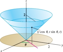
Solution A parametrization of the cone was found in Example 1. Using the variables \(\theta\) and \(t\), this parametrization is \[ {G}(\theta,t)=(t\cos\theta,t\sin\theta,t), \qquad 0\le t\le 2,\quad 0\le\theta<2\pi \]
982
Step 1. Compute the tangent and normal vectors.
\[ \begin{array}{rl} {\bf{T}}_\theta &= \frac{\partial {G}}{\partial \theta} = \left\langle -t\sin \theta, t\cos\theta , 0 \right\rangle,\qquad {\bf{T}}_t = \frac{\partial {G}}{\partial t} = \left\langle \cos\theta, \sin\theta, 1\right\rangle\\ {\bf{n}} &= {\bf{T}}_\theta{\times}{\bf{T}}_t = \left| \begin{array}{ccc} {\bf{i}} & {\bf{j}} & {\bf{k}} \\ -t\sin \theta& t\cos\theta & 0\\ \cos\theta& \sin\theta& 1 \end{array} \right| = t\cos\theta{\bf{i}}+t\sin\theta{\bf{j}}-t{\bf{k}} \end{array} \]
REMINDER
In this example, \[ {G}(\theta,t)=(t\cos\theta,t\sin\theta,t) \]
The normal vector has length \[ \left \| {\bf{n}} \right \| = \sqrt{t^2\cos^2\theta+t^2\sin^2\theta+(-t)^2}=\sqrt{2t^2}=\sqrt{2}\,|t| \]
Thus, \(dS=\sqrt{2}|t|\,d\theta\,dt\). Since \(t\geq 0\) on our domain, we drop the absolute value.
Step 2. Calculate the surface area.
\[ \textrm{Area}({\mathcal{S}}) = \iint_{{\mathcal{D}}\,} \left \| {\bf{n}} \right \|\,du\,dv = \int_0^2\int_0^{2\pi} \sqrt{2}\, t\,d\theta\,dt = \sqrt{2}\pi t^2 \bigg|_0^2 = 4\sqrt{2}\pi \]
Step 3. Calculate the surface integral.
We express \(f(x,y,z) = x^2z\) in terms of the parameters \(t\) and \(\theta\) and evaluate: \[ f({G}(\theta,t)) = f(t\cos\theta, t\sin\theta,t) = (t\cos\theta)^2t = t^3\cos^2\theta \] \[ \begin{array}{rl} \iint_{\!{\mathcal{S}}\,}f(x,y,z)\,dS &= \int_{t=0}^2\int_{\theta=0}^{2\pi} f({G}(\theta,t))\,\left \| {{\bf{n}}(\theta,t)} \right \|\,d\theta\,dt\\ &=\int_{t=0}^2\int_{\theta=0}^{2\pi} (t^3\cos^2\theta)(\sqrt{2}t)\,d\theta\,dt \\ &=\sqrt{2}\left(\int_0^2t^4\,dt\right)\left(\int_0^{2\pi}\cos^2\theta\,d\theta\right)\\ &=\sqrt{2}\left(\frac{32}5\right)(\pi) = \frac{32\sqrt{2}\pi}5 \end{array} \]
REMINDER
\[ \int_0^{2\pi} \cos^2\theta\,\,d\theta = \int_0^{2\pi}\, \frac{1+\cos 2\theta}2\,\,d\theta=\pi \]
In previous discussions of multiple and line integrals, we applied the principle that the integral of a density is the total quantity. This applies to surface integrals as well. For example, a surface with mass density \(\rho(x,y,z)\) [in units of mass per area] is the surface integral of the mass density: \[ \mathrm{Mass~of~}{\mathcal{S}} = \iint_{\!{\mathcal{S}}\,}\,\rho(x,y,z)\,dS \]
Similarly, if an electric charge is distributed over \({\mathcal{S}}\) with charge density \(\rho(x,y,z)\), then the surface integral of \(\rho(x,y,z)\) is the total charge on \({\mathcal{S}}\).
EXAMPLE 5 Total Charge on a Surface
Find the total charge (in coulombs) on a sphere \(S\) of radius 5 cm whose charge density in spherical coordinates is \(\rho(\theta,\phi) = 0.003\cos^2\phi~\text{C/cm}^2\).
Solution We parametrize \(S\) in spherical coordinates: \[ {G}(\theta,\phi)=(5\cos\theta\sin\phi,5\sin\theta\sin\phi,5\cos\phi) \]
By Eq. (2), \(\left \| {\bf{n}} \right \|=5^2\sin\phi\) and \[ \begin{array}{rl} \textrm{Total charge} &= \iint_{S\,}\rho(\theta,\phi)\,dS = \int_{\theta=0}^{2\pi}\int_{\phi=0}^{\pi}\rho(\theta,\phi)\left \| {\bf{n}} \right \|\,d\phi\,d\theta\\ &= \int_{\theta=0}^{2\pi}\int_{\phi=0}^{\pi}(0.003\cos^2\phi)(25\sin\phi)\,d\phi\,d\theta\\ &= (0.075)(2\pi)\int_{\phi=0}^{\pi} \cos^2\phi\sin\phi\,d\phi\\ &= 0.15\pi\left(-\frac{\cos^3\phi}3\right)\bigg|_0^{\pi}=0.15\pi\left(\frac23\right) \approx 0.1\pi~\mathrm{C} \end{array} \]
983
When a graph \(z=g(x,y)\) is parametrized by \({G}(x,y)=(x,y,g(x,y))\), the tangent and normal vectors are \[ {\bf{T}}_x = (1,0,g_x),\qquad {\bf{T}}_y=(0,1,g_y) \] \begin{equation*} \boxed{{\bf{n}} = {\bf{T}}_x{\times}{\bf{T}}_y = \left| \begin{array}{ccc} {\bf{i}} & {\bf{j}} & {\bf{k}} \\ 1& 0 & g_x\\ 0& 1& g_y \end{array} \right| = -g_x{\bf{i}}-g_y{\bf{j}}+{\bf{k}},\quad \left \| {\bf{n}} \right \| = \sqrt{1+g_x^2+g_y^2}}\tag{8} \end{equation*}
The surface integral over the portion of a graph lying over a domain \({\mathcal{D}}\) in the \(xy\)-plane is \begin{equation*} \boxed{\textrm{Surface integral over a graph} =\iint_{{\mathcal{D}}\,} f(x,y,g(x,y)) \sqrt{1+g_x^2+g_y^2}\, dx\, dy}\tag{9} \end{equation*}
EXAMPLE 6
Calculate \(\iint_{\!{\mathcal{S}}\,} (z-x)\,dS\), where \({\mathcal{S}}\) is the portion of the graph of \(z=x+y^2\) where \(0\le x\le y\), \(0\le y\le 1\) (Figure 16.51).
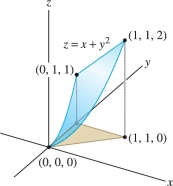
Solution Let \(z=g(x,y)=x+y^2\). Then \(g_x=1\) and \(g_y=2y\), and \[ dS = \sqrt{1+g_x^2+g_y^2}\,dx\,dy = \sqrt{1+1+4y^2}\,dx\,dy = \sqrt{2+4y^2}\,dx\,dy \]
On the surface \({\mathcal{S}}\), we have \(z =x+y^2\), and thus \[ f(x,y,z) = z-x = (x+y^2) - x = y^2 \]
By Eq. (9), \[ \begin{array}{rl} \iint_{\!{\mathcal{S}}\,} f(x,y,z)\,dS &= \int_{y=0}^1\int_{x=0}^y y^2\sqrt{2+4y^2}\,dx\,dy \\ &= \int_{y=0}^1 \left(y^2\sqrt{2+4y^2}\right)x \bigg|_{x=0}^y \,dy = \int_0^1 y^3\sqrt{2+4y^2} \, dy \end{array} \]
Now use the substitution \(u = 2+4y^2\), \(du=8y\,dy\). Then \(y^2=\tfrac14(u-2)\), and \[ \begin{array}{rl} \int_0^1 y^3\sqrt{2+4y^2} \, dy &= \frac18\int_2^6 \frac14(u-2)\sqrt{u} \, du = \frac1{32}\int_2^6(u^{3/2}-2u^{1/2})\,du\\ &= \frac1{32}\left(\frac25u^{5/2}-\frac43u^{3/2}\right)\bigg|_2^6 = \frac1{30}(6\sqrt{6} + \sqrt{2})\approx 0.54 \end{array} \]
Excursion
984
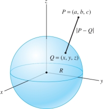
In physics it is an important fact that the gravitational field \({\bf{F}}\) corresponding to any arrangement of masses is conservative; that is, \({\bf{F}}=-\nabla{V}\) (recall that the minus sign is a convention of physics). The field at a point \(P\) due to a mass \(m\) located at point \(Q\) is \({\bf{F}}=-\frac{Gm}{r^2} {\bf{e}}_r\), where \({\bf{e}}_r\) is the unit vector pointing from \(Q\) to \(P\) and \(r\) is the distance from \(P\) to \(Q\), which we denote by \(\left | {P-Q} \right |\). As we saw in Example 4 of Section 16.3, \[ {V}(P)=-\frac{Gm}r=-\frac{Gm}{\left | {P-Q} \right |} \]
The French mathematician Pierre Simon, Marquis de Laplace (1749–1827) showed that the gravitational potential satisfies the Laplace equation \(\Delta{V} = 0\), where \(\Delta\) is the Laplace operator \[ \Delta{V} = \frac{\partial ^2{V}}{\partial x^2}+\frac{\partial ^2{V}}{\partial y^2}+\frac{\partial ^2{V}}{\partial z^2} \] This equation plays an important role in more advanced branches of math and physics.
If, instead of a single mass, we have \(N\) point masses \(m_1,\ldots,m_N\) located at \(Q_1,\ldots, Q_N\), then the gravitational potential is the sum \begin{equation*} {V}(P) = -G\sum_{i=1}^N \frac{m_i}{\left | {P-Q_i} \right |}\tag{10} \end{equation*}
If mass is distributed continuously over a thin surface \({\mathcal{S}}\) with mass density function \(\rho(x,y,z)\), we replace the sum by the surface integral \begin{equation*} {V}(P) = -G\iint_{\!{\mathcal{S}}\,} \frac{\rho(x,y,z)\,dS}{\left | {P-Q} \right |} = -G \iint_{\!{\mathcal{S}}\,} \frac{\rho(x,y,z)\,dS}{\sqrt{(x-a)^2+(y-b)^2+(z-c)^2}}\tag{11} \end{equation*} where \(P=(a,b,c)\). However, this surface integral cannot be evaluated explicitly unless the surface and mass distribution are sufficiently symmetric, as in the case of a hollow sphere of uniform mass density (Figure 16.52).
THEOREM 2 Gravitational Potential of a Uniform Hollow Sphere
The gravitational potential \({V}\) due to a hollow sphere of radius \(R\) with uniform mass distribution of total mass \(m\) at a point \(P\) located at a distance \(r\) from the center of the sphere is \begin{equation*} {V}(P) = \begin{cases} \dfrac{-Gm}{r} & \textrm{if }r>R\quad (P\textrm{ outside the sphere})\\ \dfrac{-Gm}{R} & \textrm{if }r<R\quad (P\textrm{ inside the sphere}) \end{cases}\tag{12} \end{equation*}
We leave this calculation as an exercise (Exercise 48), because we will derive it again with much less effort using Gauss’s Law in Section 17.3. In his magnum opus, Principia Mathematica, Isaac Newton proved that a sphere of uniform mass density (whether hollow or solid) attracts a particle outside the sphere as if the entire mass were concentrated at the center. In other words, a uniform sphere behaves like a point mass as far as gravity is concerned. Furthermore, if the sphere is hollow, then the sphere exerts no gravitational force on a particle inside it. Newton’s result follows from Eq.(12). Outside the sphere, \({V}\) has the same formula as the potential due to a point mass. Inside the sphere, the potential is constant with value \(-Gm/R\). But constant potential means zero force because the force is the (negative) gradient of the potential. This discussion applies equally well to the electrostatic force. In particular, a uniformly charged sphere behaves like a point charge (when viewed from outside the sphere).
16.4.1 Summary
985
- A parametrized surface is a surface \({\mathcal{S}}\) whose points are described in the form \[ {G}(u,v)=(x(u,v), y(u,v),z(u,v)) \] where the parameters \(u\) and \(v\) vary in a domain \({\mathcal{D}}\) in the \(uv\)-plane.
- Tangent and normal vectors: \[ \begin{array}{rl} {\bf{T}}_u &= \frac{\partial {G}}{\partial u} = \left\langle \frac{\partial x}{\partial u} ,\frac{\partial y}{\partial u} ,\frac{\partial z}{\partial u}\right\rangle,\qquad{\bf{T}}_v = \frac{\partial {G}}{\partial v} = \left\langle \frac{\partial x}{\partial v} ,\frac{\partial y}{\partial v},\frac{\partial z}{\partial v}\right\rangle\\ {\bf{n}} &= {\bf{n}}(u,v) = {\bf{T}}_u{\times}{\bf{T}}_v \end{array} \] The parametrization is regular at \((u,v)\) if \({\bf{n}}(u,v)\ne \mathbf{0}\).
- The quantity \(\left \| {\bf{n}} \right \|\) is an “area distortion factor.” If \({\mathcal{D}}\) is a small region in the \(uv\)-plane and \({\mathcal{S}}={G}({\mathcal{D}})\), then \[ \textrm{Area}({\mathcal{S}}) \approx \left \| {{\bf{n}}(u_0,v_0)} \right \|\textrm{Area}({\mathcal{D}}) \] where \((u_0,v_0)\) is any sample point in \({\mathcal{D}}\).
- Formulas: \[ \begin{array}{rl} \textrm{Area}({\mathcal{S}}) &= \iint_{{\mathcal{D}}\,} \left \| {{\bf{n}}(u,v)} \right \|\,du\,dv\\ \iint_{\!{\mathcal{S}}\,}\,f(x,y,z)\,dS &= \iint_{{\mathcal{D}}\,} f({G}(u,v))\, \left \| {{\bf{n}}(u,v)} \right \|\,du\,dv \end{array} \]
- Some standard parametrizations:
- Cylinder of radius \(R\) (\(z\)-axis as central axis): \[ \begin{array}{rl} &{G}(\theta,z) = (R\cos\theta, R\sin\theta, z)\\ &\textrm{Outward normal:} \quad{\bf{n}} ={\bf{T}}_\theta{\times}{\bf{T}}_z = R\left\langle \cos \theta, \sin\theta, 0 \right\rangle\\ &dS =\left \| {\bf{n}} \right \|\,d\theta\,dz = R\,d\theta\,dz \end{array} \]
- Sphere of radius \(R\), centered at the origin: \[ \begin{array}{rl} &{G}(\theta,\phi) = (R\cos\theta\sin\phi, R\sin\theta\sin\phi, R\cos\phi)\\ &\textrm{Unit radial vector:} \quad{\bf{e}}_r = \left\langle \cos\theta\sin\phi, \sin\theta\sin\phi, \cos\phi \right\rangle \\ &\textrm{Outward normal:} \quad{\bf{n}} ={\bf{T}}_\phi {\times}{\bf{T}}_\theta= (R^2 \sin\phi)\,{\bf{e}}_r\\ &dS=\left \| {\bf{n}} \right \|\,d\phi\,d\theta = R^2\sin\phi\,d\phi\,d\theta \end{array} \]
- Graph of \(z=g(x,y)\): \[ \begin{array}{rl} &{G}(x,y) = (x,y,g(x,y))\\ &{\bf{n}} = {\bf{T}}_x{\times}{\bf{T}}_y=\left\langle -g_x,-g_y,1\right\rangle\\ &dS=\left \| {\bf{n}} \right \|\,dx\, dy =\sqrt{1+g_x^2+g_y^2}\,dx\, dy \end{array} \]