17.2 Green’s Theorem
In Section 16.3, we showed that the circulation of a conservative vector field \({\bf F}\) around every closed path is zero. For vector fields in the plane, Green’s Theorem tells us what happens when \({\bf F}\) is not conservative.
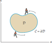
To formulate Green’s Theorem, we need some notation. Consider a domain \(D\) whose boundary \(C\) is a simple closed curve—that is, a closed curve that does not intersect itself (Figure 17.1). We follow standard usage and denote the boundary curve \(C\) by \(\partial D\). The counterclockwise orientation of \(\partial D\) is called the boundary orientation. When you traverse the boundary in this direction, the domain lies to your left (Figure 17.1).
Recall that we have two notations for the line integral of \({\bf F} = \langle F_1,F_2\rangle\): \[ \int_{C}{\bf F}\cdot d{\bf s}\qquad\textrm{and}\qquad \int_{C}F_1\, dx + F_2\,dy \]
If \(C\) is parametrized by \(c(t)=(x(t),y(t))\) for \(a \leq t \leq b\), then \begin{array} dx=x'(t)\,dt,\qquad dy=y'(t)\,dt\\ \int_{C} F_1 \, dx + F_2 \,dy = \int_a^b \left( F_1(x(t),y(t))x'(t) + F_2(x(t),y(t))y'(t) \right)\,dt\tag{1} \end{array}
Throughout this chapter, we assume that the components of all vector fields have continuous partial derivatives, and also that \(C\) is smooth (\(C\) has a parametrization with derivatives of all orders) or piecewise smooth (a finite union of smooth curves joined together at corners).
REMINDER
The line integral of a vector field over a closed curve is called the “circulation” and is often denoted with the symbol \(\displaystyle{\oint}\).
THEOREM 1 Green’s Theorem
Let \(D\) be a domain whose boundary \(\partial D\) is a simple closed curve, oriented counterclockwise. Then \begin{equation} \boxed{\oint_{\partial D} F_1\,dx+F_2\,dy = \iint_{D\,}\left(\dfrac{\partial{F_2}}{\partial{x}}-\dfrac{\partial{F_1}}{\partial {y}}\right)\,dA}\tag{2} \end{equation}
1004
Proof
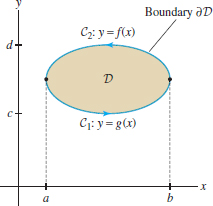
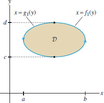
Because a complete proof is quite technical, we shall make the simplifying assumption that the boundary of \(D\) can be described as the union of two graphs \(y=g(x)\) and \(y=f(x)\) with \(g(x)\le f(x)\) as in Figure 17.2 and also as the union of two graphs \(x=g_1(y)\) and \(x=f_1(y)\), with \(g_1(y)\le f_1(y)\) as in Figure 17.3.
Green’s Theorem splits up into two equations, one for \(F_1\) and one for \(F_2\): \begin{align} \oint_{\partial D} F_1\,dx &= - \iint_{D\,} \dfrac{\partial{F_1}}{\partial {y}}\,dA \tag{3}\\ \oint_{\partial D} F_2\,dy &= \iint_{D\,}\dfrac{\partial{F_2}}{\partial{x}}\,dA\tag{4} \end{align}
In other words, Green’s Theorem is obtained by adding these two equations. To prove Eq. (3), we write \[ \oint_{\partial D} F_1\,dx = \oint_{C_1} F_1\,dx + \oint_{C_2} F_1\,dx \] where \(C_1\) is the graph of \(y=g(x)\) and \(C_2\) is the graph of \(y=f(x)\), oriented as in Figure 17.2. To compute these line integrals, we parameterize the graphs from left to right using \(t\) as parameter: \begin{align*} &\mathrm{Graph of\ } y=g(x){:} &\qquad \mathbf{c}_1(t)=(t, g(t)), &\qquad &a\le t \le b\\ &\mathrm{Graph of\ } y=f(x){:} &\qquad \mathbf{c}_2(t)=(t, f(t)), &\qquad &a\le t \le b \end{align*}
Since \(C_2\) is oriented from right to left, the line integral over \(\partial D\) is the difference \begin{eqnarray*} \oint_{\partial D} F_1\,dx &=& \int_{\mathbf{c}_1} F_1\,dx - \int_{\mathbf{c}_2} F_1\,dx \end{eqnarray*}
In both parametrizations, \(x=t\), so \(dx = dt\), and by Eq. (1) \begin{equation} \oint_{\partial D} F_1\,dx = \int_{t=a}^b F_1(t,g(t))\,dt - \int_{t=a}^b F_1(t,f(t))\,dt\tag{5} \end{equation}
Now, the key step is to apply the Fundamental Theorem of Calculus to \(\dfrac{\partial{F_1}}{\partial {y}}(t,y)\) as a function of \(y\) with \(t\) held constant: \[ F_1(t, f(t)) - F_1(t, g(t)) = \int_{y=g(t)}^{f(t)} \dfrac{\partial{F_1}}{\partial {y}}(t,y)\,dy \]
Substituting the integral on the right in Eq. (5), we obtain Eq. (3): \[ \oint_{\partial D} F_1\,dx = -\int_{t=a}^b\int_{y=g(t)}^{f(t)} \dfrac{\partial{F_1}}{\partial {y}}(t,y)\,dy\,dt = -\iint_{D\,} \dfrac{\partial{F_1}}{\partial {y}}\,dA \]
Eq. (4) is proved in a similar fashion, by expressing \(\partial D\) as the union of the graphs of \(x=f_1(y)\) and \(x=g_1(y)\) (Figure 17.3).
Recall that if \({\bf F}=\nabla V\), then the cross-partial condition is satisfied: \[ \dfrac{\partial{F_2}}{\partial{x}}-\dfrac{\partial{F_1}}{\partial {y}}=0 \]
In this case, Green’s Theorem merely confirms what we already know: The line integral of a conservative vector field around any closed curve is zero.
1005
EXAMPLE 1 Verifying Green’s Theorem
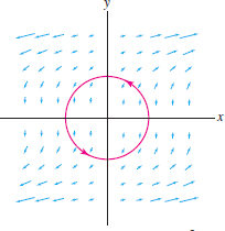
Verify Green’s Theorem for the line integral along the unit circle \(C\), oriented counterclockwise (Figure 17.4): \[ \oint_C xy^2\,dx + x\, dy \]
Solution
Step 1. Evaluate the line integral directly.
We use the standard parametrization of the unit circle: \begin{align*} x &= \cos\theta,&\qquad y &= \sin\theta \\ dx &= -\sin\theta\,d\theta,&\qquad dy &= \cos\theta\,d\theta \end{align*}
Note
Green’s Theorem states: \begin{multline*} \oint_{\partial D} F_1\,dx+F_2\,dy\\ = \iint_{D\,}\left(\dfrac{\partial{F_2}}{\partial{x}}-\dfrac{\partial{F_1}}{\partial {y}}\right)\,dA \end{multline*}
The integrand in the line integral is \begin{align*} xy^2\,dx + x\,dy &= \cos\theta\sin^2\theta(-\sin\theta\,d\theta)+\cos\theta (\cos\theta\,d\theta)\\ &= \bigl(-\cos\theta\sin^3\theta +\cos^2\theta \bigr)\,d\theta \end{align*} and \begin{align*} \oint_C xy^2\,dx + x\,dy &= \int_0^{2\pi} \bigl(-\cos\theta\sin^3\theta +\cos^2\theta \bigr)\,d\theta\\ &= -\frac{\sin^4\theta}4\bigg|_0^{2\pi} + \frac12\left(\theta+\frac12\sin 2\theta\right)\bigg|_0^{2\pi}\\ &= 0 + \frac12(2\pi + 0) = \boxed{\pi} \end{align*}
REMINDER
To integrate \(\cos^2\theta\), use the identity \(\cos^2\theta =\tfrac12(1+\cos2\theta)\).
Step 2. Evaluate the line integral using Green’s Theorem.
In this example, \(F_1=xy^2\) and \(F_2=x\), so \[ \dfrac{\partial{F_2}}{\partial{x}}-\dfrac{\partial{F_1}}{\partial{y}} = \dfrac{\partial}{\partial{x}} x - \dfrac{\partial}{\partial{y}} xy^2 = 1-2xy \]
According to Green’s Theorem, \[ \oint_C xy^2\,dx + x\,dy = \iint_{D\,} \left(\dfrac{\partial{F_2}}{\partial{x}}-\dfrac{\partial{F_1}}{\partial{y}}\right)\,dA = \iint_{D\,}(1-2xy)\,dA \] where \(D\) is the disk \(x^2+y^2\le 1\) enclosed by \(C\). The integral of \(2xy\) over \(D\) is zero by symmetry—the contributions for positive and negative \(x\) cancel. We can check this directly: \[ \iint_{D\,} (-2xy)\,dA = -2 \int_{x=-1}^1\, \int_{y=-\sqrt{1-x^2}}^{\sqrt{1-x^2}}xy\,dy\,dx = - \int_{x=-1}^1\, xy^2\Big|_{y=-\sqrt{1-x^2}}^{\sqrt{1-x^2}}\,dx = 0 \] Therefore, \[ \iint_{D\,} \left(\dfrac{\partial{F_2}}{\partial{x}}-\dfrac{\partial{F_1}}{\partial{y}}\right)\,dA = \iint_{D\,} 1\,dA = \textrm{Area}(D) = \boxed{\pi} \]
This agrees with the value in Step 1, so Green’s Theorem is verified in this case.
EXAMPLE 2 Computing a Line Integral Using Green’s Theorem
Compute the circulation of \(\displaystyle{{\bf F} =0 \langle \sin x,x^2y^3\rangle}\) around the triangular path \(C\) in Figure 17.5.
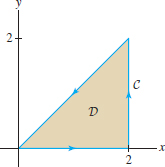
Solution To compute the line integral directly, we would have to parametrize all three sides of the triangle. Instead, we apply Green’s Theorem to the domain \(D\) enclosed by the triangle. This domain is described by \(0\le x \le 2\), \(0\le y \le x\).
1006
Applying Green’s Theorem, we obtain \[\dfrac{\partial{F_2}}{\partial{x}}-\dfrac{\partial{F_1}}{\partial{y}} = \dfrac{\partial}{\partial{x}}\,x^2y^3-\dfrac{\partial}{\partial{y}}\,\sin x = 2xy^3\] \begin{align*} \oint_C \sin x\,dx+ x^2y^3\,dy &= \iint_{D\,} 2xy^3\,dA = \int_0^2\int_{y=0}^x 2xy^3\,dy\,dx\\ & = \int_0^2 \left(\frac12xy^4\bigg|_0^x\right)\,dx = \frac12\int_0^2 x^5\,dx = \frac1{12}x^6\bigg|_0^2 = \frac{16}3 \end{align*}
Green’s Theorem applied to \({\bf F} = \langle -y,x\rangle\) leads to a formula for the area of the domain \(D\) enclosed by a simple closed curve \(C\) (Figure 17.6). We have \begin{align*} & \dfrac{\partial{F_2}}{\partial{x}}-\dfrac{\partial{F_1}}{\partial{y}} = \dfrac{\partial}{\partial{x}} x -\dfrac{\partial}{\partial{y}} (-y)=2 \end{align*}
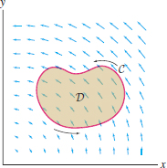
By Green’s Theorem, \(\displaystyle{ \oint_C -y\,dx+x\,dy = \iint_{D\,} 2\,dx\,dy = 2\,\textrm{Area}(D)}\). We obtain \begin{equation} \boxed{ \textrm{Area enclosed by \(C\)} = \frac{1}{2}\oint_C x\,dy-y\,dx}\tag{6} \end{equation}
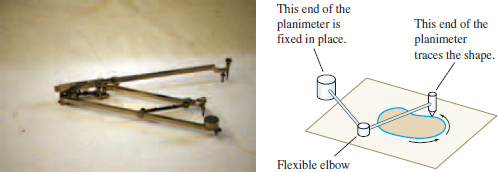
This remarkable formula tells us how to compute an enclosed area by making measurements only along the boundary. It is the mathematical basis of the planimeter, a device that computes the area of an irregular shape when you trace the boundary with a pointer at the end of a movable arm (Figure 17.7).
EXAMPLE 3 Computing Area via Green’s Theorem
Compute the area of the ellipse \(\displaystyle{\left(\frac{x}a\right)^2+\left(\frac{y}b\right)^2=1}\) using a line integral.
Note
“Fortunately (for me), I was the only one in the local organization who had even heard of Green’s Theorem,...although I was not able to make constructive contributions, I could listen, nod my head and exclaim in admiration at the right places.” John M. Crawford, geophysicist and director of research at Conoco Oil, 1951–1971, writing about his first job interview in 1943, when a scientist visiting the company began speaking about applications of mathematics to oil exploration.
Solution
We parametrize the boundary of the ellipse by \[ x=a\cos\theta,\qquad y=b\sin\theta,\qquad 0 \le \theta < 2\pi \] and use Eq. (6): \begin{align*} x\,dy -y\,dx &= (a\cos\theta)(b\cos\theta\,d\theta) - (b\sin\theta)(-a\sin\theta\,d\theta)\\ &=ab(\cos^2\theta + \sin^2\theta)\,d\theta=ab\,d\theta\\ \textrm{Enclosed area} &= \frac12\oint_C x\,dy - y\,dx = \frac12\int_0^{2\pi} ab\,d\theta=\pi ab \end{align*}
This is the standard formula for the area of an ellipse.
1007
CONCEPTUAL INSIGHT
What is the meaning of the integrand in Green’s Theorem? For convenience, we denote this integrand by \({\bf curl}_z({\bf F})\): \[ {\bf curl}_z({\bf F}) = \dfrac{\partial{F_2}}{\partial{x}}-\dfrac{\partial{F_1}}{\partial{y}} \]
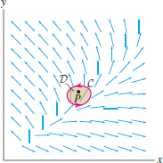
In Section 17.3, we will see that \({\bf curl}_z({\bf F})\) is the \(z\)-component of a vector field \({\bf curl}({\bf F})\) called the “curl” of \({\bf F}\). Now apply Green’s Theorem to a small domain \(D\) with simple closed boundary curve and let \(P\) be a point in \(D\). Because \({\bf curl}_z({\bf F})\) is a continuous function, its value does not change much on \(D\) if \(C\) is sufficiently small, so to a first approximation, we can replace \({\bf curl}_z({\bf F})\) by the constant value \({\bf curl}_z({\bf F})(P)\) (Figure 17.8). Green’s Theorem yields the following approximation for the circulation: \begin{align} \oint_C {\bf F}\cdot d{\bf s} &= \iint_{D\,}{\bf curl}_z({\bf F})\,dA\notag\\ & \approx {\bf curl}_z({\bf F})(P)\iint_{D\,}\,dA\notag\\ &\approx {\bf curl}_z({\bf F})(P) \cdot \textrm{Area}(D)\tag{7} \end{align}
In other words, the circulation around a small, simple closed curve \(C\) is, to a first-order approximation, equal to the curl times the enclosed area. Thus, we can think of \(\displaystyle{{\bf curl}_z({\bf F})(P)}\) as the circulation per unit of enclosed area.
Angular Velocity
An arc of \(\ell\) meters on a circle of radius \(r\) meters has radian measure \(\ell/r\). Therefore, an object moving along the circle with a speed of \(v\) meters per second travels \(v/r\) radians per second. In other words, the object has angular velocity \(v/r\).
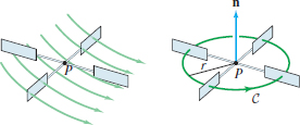
GRAPHICAL INSIGHT
If we think of \({\bf F}\) as the velocity field of a fluid, then we can measure the curl by placing a small paddle wheel in the stream at a point \(P\) and observing how fast it rotates (Figure 17.9). Because the fluid pushes each paddle to move with a velocity equal to the tangential component of \({\bf F}\), we can assume that the wheel itself rotates with a velocity \(v_a\) equal to the average tangential component of \({\bf F}\). If the paddle is a circle \(C\) of radius \(r\) (and hence length \(2\pi r\)), then the average tangential component of velocity is \[ v_a = \frac1{2 \pi r}\oint_{C_r} {\bf F}\cdot d{\bf s} \] On the other hand, the paddle encloses an area of \(\pi r^2\), and for small \(r\), we can apply the approximation (7): \[ v_a \approx \frac1{2 \pi r} (\pi r^2){\bf curl}_z({\bf F})(P) = \left(\frac12r\right) {\bf curl}_z({\bf F})(P) \] Now if an object moves along a circle of radius \(r\) with speed \(v_a\), then its angular velocity (in radians per unit time) is \(v_a/r\approx\frac12{\bf curl}_z({\bf F})(P)\). Therefore, the angular velocity of the paddle wheel is approximately one-half the curl.
1008
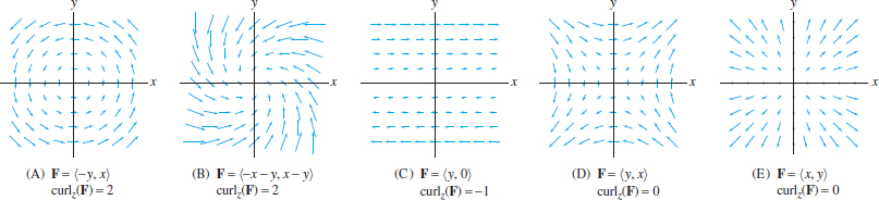
Figure 17.10 shows vector fields with constant curl. Field (A) describes a fluid rotating counterclockwise around the origin, and field (B) describes a fluid that spirals into the origin. However, a nonzero curl does not mean that the fluid itself is necessarily rotating. It means only that a small paddle wheel would rotate if placed in the fluid. Field (C) is an example of shear flow (also known as a Couette flow). It has nonzero curl but does not rotate about any point. Compare with the fields in Figures (D) and (E), which have zero curl.
Additivity of Circulation
Circulation around a closed curve has an important additivity property: If we decompose a domain \(D\) into two (or more) non-overlapping domains \(D_1\) and \(D_2\) that intersect only on part of their boundaries as in Figure 17.11, then \begin{equation} \boxed{ \oint_{\partial D}{\bf F}\cdot d{\bf s} = \oint_{\partial D_1}{\bf F}\cdot d{\bf s} + \oint_{\partial D_2}{\bf F}\cdot d{\bf s}}\tag{8} \end{equation}
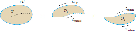
To verify this equation, note first that \[ \oint_{\partial D}{\bf F}\cdot d{\bf s} = \int_{C_{\mathrm{top}}}{\bf F}\cdot d{\bf s} + \int_{C_{\mathrm{bot}}}{\bf F}\cdot d{\bf s} \] with \(C_{\mathrm{top}}\) and \(C_{\mathrm{bot}}\) as in Figure 11. Then observe that the dashed segment \(C_{\mathrm{middle}}\) occurs in both \(\partial D_1\) and \(\partial D_2\) but with opposite orientations. If \(C_{\mathrm{middle}}\) is oriented right to left, then \begin{align*} \oint_{\partial D_1}{\bf F}\cdot d{\bf s} &= \int_{C_{\mathrm{top}}}{\bf F}\cdot d{\bf s} - \int_{C_{\mathrm{middle}}}{\bf F}\cdot d{\bf s}\\ \oint_{\partial D_2}{\bf F}\cdot d{\bf s} &= \int_{C_{\mathrm{bot}}}{\bf F}\cdot d{\bf s} + \int_{C_{\mathrm{middle}}}{\bf F}\cdot d{\bf s} \end{align*}
We obtain Eq. (8) by adding these two equations: \[ \oint_{\partial D_1} {\bf F} \cdot d{\bf s} + \oint_{\partial D_2} {\bf F} \cdot d{\bf s} = \int_{C_{\mathrm{top}}} {\bf F} \cdot d{\bf s} + \int_{C_{\mathrm{bot}}} {\bf F} \cdot d{\bf s} = \oint_{\partial D} {\bf F} \cdot d{\bf s} \]
1009
More General Form of Green’s Theorem
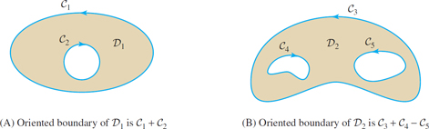
Consider a domain \(D\) whose boundary consists of more than one simple closed curve as in Figure 17.12. As before, \(\partial D\) denotes the boundary of \(D\) with its boundary orientation. In other words, the region lies to the left as the curve is traversed in the direction specified by the orientation. For the domains in Figure 17.12, \[ \partial D_1 = C_1+C_2,\qquad \partial D_2 = C_3+C_4 - C_5 \]
The curve \(C_5\) occurs with a minus sign because it is oriented counterclockwise, but the boundary orientation requires a clockwise orientation.
Green’s Theorem remains valid for more general domains of this type: \begin{equation} \boxed{ \oint_{\partial D} {\bf F}\cdot d{\bf s} = \iint_{D\,} \left(\dfrac{\partial{F_2}}{\partial{x}}-\dfrac{\partial{F_1}}{\partial{y}}\right)\,dA}\tag{9} \end{equation}
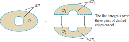
This equality is proved by decomposing \(D\) into smaller domains each of which is bounded by a simple closed curve. To illustrate, consider the region \(D\) in Figure 17.13. We decompose \(D\) into domains \(D_1\) and \(D_2\). Then \[ \partial D = \partial D_1 + \partial D_2 \] because the edges common to \(\partial D_1\) and \(\partial D_2\) occur with opposite orientation and therefore cancel. The previous version of Green’s Theorem applies to both \(D_1\) and \(D_2\), and thus \begin{align*} \oint_{\partial D}{\bf F}\cdot d{\bf s} &=\int_{\partial D_1}{\bf F}\cdot d{\bf s}+\int_{\partial D_2}{\bf F}\cdot d{\bf s} \\& =\iint_{D_1\,}\left(\dfrac{\partial{F_2}}{\partial{x}}-\dfrac{\partial{F_1}}{\partial{y}}\right)\,dA + \iint_{D_2\,}\left(\dfrac{\partial{F_2}}{\partial{x}}-\dfrac{\partial{F_1}}{\partial{y}}\right)\,dA\\ &=\iint_{D\,}\left(\dfrac{\partial{F_2}}{\partial{x}}-\dfrac{\partial{F_1}}{\partial{y}}\right)\,dA \end{align*}
1010
EXAMPLE 4
Calculate \(\displaystyle{\oint_{C_1} {\bf F}\cdot d{\bf s}}\), where \({\bf F} = \langle x-y, x+y^3\rangle\) and \(C_1\) is the outer boundary curve oriented counterclockwise. Assume that the domain \(D\) in Figure 17.14 has area 8.
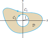
Solution We cannot compute the line integral over \(C_1\) directly because the curve \(C_1\) is not specified. However, \(\partial D =C_1-C_2\), so Green’s Theorem yields \begin{equation} \oint_{C_1}{\bf F}\cdot d{\bf s}-\oint_{C_2}{\bf F}\cdot d{\bf s} = \iint_{D\,}\left(\dfrac{\partial{F_2}}{\partial{x}}-\dfrac{\partial{F_1}}{\partial{y}}\right)\,dA\tag{10} \end{equation}
We have \begin{align*} \dfrac{\partial{F_2}}{\partial{x}}-\dfrac{\partial{F_1}}{\partial{y}} &= \dfrac{\partial}{\partial{x}}(x+y^3) -\dfrac{\partial}{\partial{y}}(x-y) = 1- (-1)= 2\\ \iint_{D\,}\left(\dfrac{\partial{F_2}}{\partial{x}}-\dfrac{\partial{F_1}}{\partial{y}}\right)\,dA &= \iint_{D\,}\,2\,dA = 2\,\textrm{Area}(D) = 2(8)=16 \end{align*}
Thus Eq. (10) gives us \begin{equation} \oint_{C_1}{\bf F}\cdot d{\bf s} - \oint_{C_2}{\bf F}\cdot d{\bf s} = 16\tag{11} \end{equation}
To compute the second integral, parametrize the unit circle \(C_2\) by \({\bf c}(t)=(\cos\theta, \sin\theta)\). Then \begin{align*} {\bf F}\cdot{\bf c}'(t) &= \langle \cos\theta-\sin\theta, \cos\theta+\sin^3\theta \rangle\cdot\langle -\sin\theta, \cos\theta\rangle\\ & = -\sin\theta\cos\theta+\sin^2\theta+\cos^2\theta+\sin^3\theta\cos\theta \\&=1-\sin\theta\cos\theta+\sin^3\theta\cos\theta \end{align*}
The integrals of \(\sin\theta\cos\theta\) and \(\sin^3\theta\cos\theta\) over \([0,2\pi]\) are both zero, so \[ \oint_{C_2}{\bf F} \cdot d{\bf s} = \int_0^{2\pi} (1-\sin\theta\cos\theta+\sin^3\theta\cos\theta)\,d\theta = \int_0^{2\pi} d\theta = 2\pi \]
Eq. (11) yields \({\oint_{C_1} {\bf F}\cdot d{\bf s} = 16 +2\pi}\).