9.3 Graphical and Numerical Methods
In the previous two sections, we focused on finding solutions to differential equations. However, most differential equations cannot be solved explicitly. Fortunately, there are techniques for analyzing the solutions that do not rely on explicit formulas. In this section, we discuss the method of slope fields, which provides us with a good visual understanding of first-order equations. We also discuss Euler's Method for finding numerical approximations to solutions.
“To imagine yourself subject to a differential equation, start somewhere. There you are tugged in some direction, so you move that way ... as you move, the tugging forces change, pulling you in a new direction; for your motion to solve the differential equation you must keep drifting with and responding to the ambient forces.”
—From the introduction to Differential Equations, J. H. Hubbard and Beverly West, Springer-Verlag, New York, 1991
We use \(t\) as the independent variable and write \(\dot{y}\) for \({dy}/{dt}\). The notation \(\dot{y}\), often used for time derivatives in physics and engineering, was introduced by Isaac Newton. A first-order differential equation can then be written in the form \[ \begin{equation} \boxed{\bbox[#FAF8ED,5pt]{\dot{y} = F(t,y)}} \end{equation}\tag {1} \] where \(F(t,y)\) is a function of \(t\) and \(y\). For example, \(\displaystyle dy/dt = ty\) becomes \(\dot{y}= ty\).
517
It is useful to think of Eq.(1) as a set of instructions that “tells a solution” which direction to go in. Thus, a solution passing through a point \((t,y)\) is “instructed” to continue in the direction of slope \(F(t,y)\). To visualize this set of instructions, we draw a slope field, which is an array of small segments of slope \(F(t,y)\) at points \((t,y)\) lying on a rectangular grid in the plane.
To illustrate, let's return to the differential equation: \[ \dot{y}=-ty \]
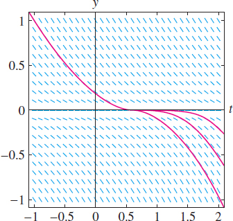
In this case, \(F(t,y) = -ty\). According to Example 2 of Section 9.1, the general solution is \(y=Ce^{-t^2/2}\). Figure 9.12 shows segments of slope \(-ty\) at points \((t,y)\) along the graph of a particular solution \(y(t)\). This particular solution passes through \((-1,3)\), and according to the differential equation, \(\dot{y}(-1)=-ty = -(-1)3=3\). Thus, the segment located at the point \((-1,3)\) has slope 3. The graph of the solution is tangent to each segment [Figure 9.12].
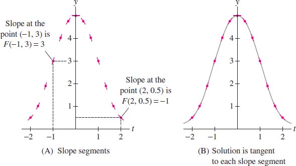
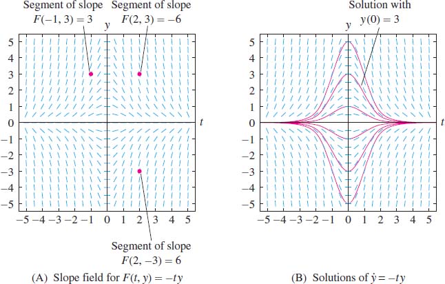
To sketch the slope field for \(\dot{y}=-ty\), we draw small segments of slope \(-ty\) at an array of points \((t, y)\) in the plane, as in Figure 9.13 The slope field allows us to visualize all of the solutions at a glance. Starting at any point, we can sketch a solution by drawing a curve that runs tangent to the slope segments at each point [Figure 9.13]. The graph of a solution is also called an integral curve.
518
EXAMPLE 1 Using Isoclines
Draw the slope field for \[\dot{y}=y-t\] and sketch the integral curves satisfying the initial conditions (a) \(y(0) = 1\) and (b) \(y(1) = -2\).
Solution
A good way to sketch the slope field of \(\dot{y} = F(t, y)\) is to choose several values \(c\) and identify the curve \(F(t,y)=c\), called the isocline of slope \(c\). The isocline is the curve consisting of all points where the slope field has slope \(c\).
In our case, \(F(t,y)=y-t\), so the isocline of fixed slope \(c\) has equation \(y-t=c\), or \(y = t+c\), which is a line. Consider the following values:
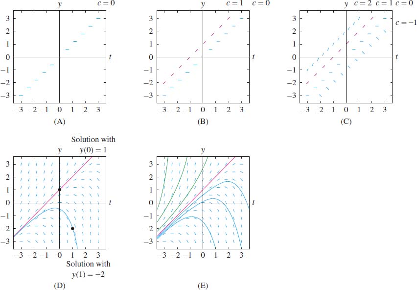
- \(c = 0\): This isocline is \(y -t = 0\), or \(y=t\). We draw segments of slope \(c=0\) at points along the line \(y=t\), as in Figure 9.14.
- \(c = 1\): This isocline is \(y -t = 1\), or \(y=t+1\). We draw segments of slope \(1\) at points along \(y=t+1\), as in Figure 9.14.
- \(c = 2\): This isocline is \(y -t = 2\), or \(y=t+2\). We draw segments of slope \(2\) at points along \(y=t+2\), as in Figure 9.14.
- \(c = -1\): This isocline is \(y -t = -1\), or
\(y=t-1\) [Figure 9.14.
A more detailed slope field is shown in Figure 9.14. To sketch the solution satisfying \(y(0) = 1\), begin at the point \((t_0,y_0) = (0,1)\) and draw the integral curve that follows the directions indicated by the slope field. Similarly, the graph of the solution satisfying \(y(1) = -2\) is the integral curve obtained by starting at \((t_0,y_0) = (1,-2)\) and moving along the slope field. Figure 9.14 shows several other solutions (integral curves).
519
GRAPHICAL INSIGHT
Slope fields often let us see the asymptotic behavior of solutions (as \(t\to\infty\)) at a glance. Figure 9.14 suggests that the asymptotic behavior depends on the initial value (the \(y\)-intercept): If \(y(0)>1\), then \(y(t)\) tends to \(\infty\), and if \(y(0)<1\), then \(y(t)\) tends to \(-\infty\). We can check this using the general solution \(y(t) = 1 + t + Ce^t\), where \(y(0)=1+C\). If \(y(0)>1\), then \(C>0\) and \(y(t)\) tends to \(\infty\), but if \(y(0)<1\), then \(C<0\) and \(y(t)\) tends to \(-\infty\). The solution \(y=1+t\) with initial condition \(y(0)=1\) is the straight line shown in Figure 9.14.
EXAMPLE 2 Newton's Law of Cooling Revisited
The temperature \(y(t)\)(\(^\circ\)C) of an object placed in a refrigerator satisfies \(\dot{y} = -0.5(y-4)\)(\(t\) in minutes). Draw the slope field and describe the behavior of the solutions.
Solution
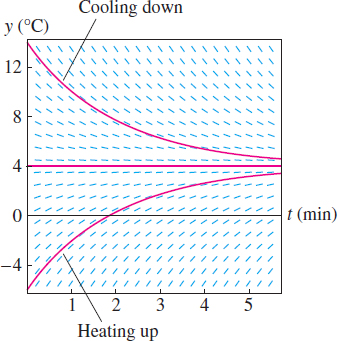
The function \(F(t,y)=-0.5(y-4)\) depends only on \(y\), so slopes of the segments in the slope field do not vary in the \(t\)-direction. The slope \(F(t,y)\) is positive for \(y<4\) and negative for \(y>4\). More precisely, the slope at height \(y\) is \(-0.5(y - 4) = -0.5y + 2\), so the segments grow steeper with positive slope as \(y\to -\infty\), and they grow steeper with negative slope as \(y\to \infty\) (Figure 9.15).
The slope field shows that if the initial temperature satisfies \(y_0>4\), then \(y(t)\) decreases to \(y=4\) as \(t\to\infty\). In other words, the object cools down to \(4^\circ\)C when placed in the refrigerator. If \(y_0<4\), then \(y(t)\) increases to \(y=4\) as \(t\to\infty-\) the object warms up when placed in the refrigerator. If \(y_0 = 4\), then \(y\) remains at \(4^\circ\)C for all time \(t\).
CONCEPTUAL INSIGHT
Most first-order equations arising in applications have a uniqueness property: There is precisely one solution \(y(t)\) satisfying a given initial condition \(y(t_0) = y_0\). Graphically, this means that precisely one integral curve (solution) passes through the point \((t_0,y_0)\). Thus, when uniqueness holds, distinct integral curves never cross or overlap. Figure 9.16 shows the slope field of \(\dot{y}=-\sqrt{|y|}\), where uniqueness fails. We can prove that once an integral curve touches the \(t\)-axis, it either remains on the \(t\)-axis or continues along the \(t\)-axis for a period of time before moving below the \(t\)-axis. Therefore, infinitely many integral curves pass through each point on the \(t\)-axis. However, the slope field does not show this clearly. This highlights again the need to analyze solutions rather than rely on visual impressions alone.
Euler's Method
Euler's Method produces numerical approximations to the solution of a first-order initial value problem: \[ \begin{equation} \dot{y}=F(t,y),\qquad y(t_0)=y_0 \tag {2} \end{equation} \]
Euler's Method is the simplest method for solving initial value problems numerically, but it is not very efficient. Computer systems use more sophisticated schemes, making it possible to plot and analyze solutions to the complex systems of differential equations arising in areas such as weather prediction, aerodynamic modeling, and economic forecasting.
We begin by choosing a small number \(h\), called the time step, and consider the sequence of times spaced at intervals of size \(h\): \[ t_0,\qquad t_1=t_0+h,\qquad t_2=t_0+2h,\qquad t_3=t_0+3h,\qquad \ldots \]
In general, \(t_k = t_0+kh\). Euler's Method consists of computing a sequence of values \(y_1, y_2, y_3, \ldots, y_n\) successively using the formula \[ \begin{equation} \boxed{\bbox[#FAF8ED,5pt]{y_k = y_{k-1}+hF(t_{k-1},y_{k-1})}} \tag {3} \end{equation} \]
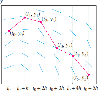
Starting with the initial value \(y_0 = y(t_0)\), we compute \(y_1 = y_0+hF(t_0,y_0)\), etc. The value \(y_k\) is the Euler approximation to \(y(t_k)\). We connect the points \(P_k= (t_k,y_k)\) by segments to obtain an approximation to the graph of \(y(t)\) (Figure 9.17).
520
GRAPHICAL INSIGHT
The values \(y_k\) are defined so that the segment joining \(P_{k-1}\) to \(P_k\) has slope \[ \frac{y_k - y_{k-1}}{t_k-t_{k-1}} = \frac{(y_{k-1}+hF(t_{k-1},y_{k-1})) - y_{k-1}}h = F(t_{k-1},y_{k-1}) \] Thus, in Euler's method we move from \(P_{k-1}\) to \(P_k\) by traveling in the direction specified by the slope field at \(P_{k-1}\) for a time interval of length \(h\)(Figure 9.17).
EXAMPLE 3
Use Euler's Method with time step \(h=0.2\) and \(n=4\) steps to approximate the solution of \(\dot{y}=y-t^2\), \(y(0)=3\).
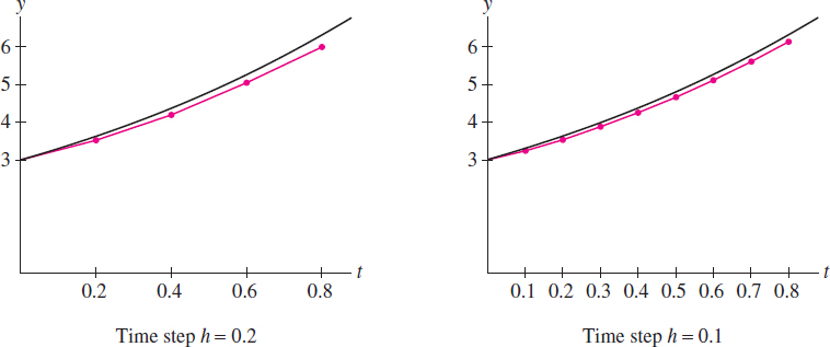
Solution Our initial value at \(t_0 = 0\) is \(y_0=3\). Since \(h=0.2\), the time values are \(t_1 = 0.2\), \(t_2=0.4\), \(t_3=0.6\), and \(t_4=0.8\). We use Eq. (3) with \(F(t,y) = y - t^2\) to calculate \[ \begin{align*} y_1 &= y_0+hF(t_0,y_0) = 3 + 0.2(3-(0)^2) = 3.6\\ y_2 &= y_1+hF(t_1,y_1) = 3.6 + 0.2(3.6-(0.2)^2) \approx 4.3\\ y_3 &= y_2+hF(t_2,y_2) = 4.3 + 0.2(4.3-(0.4)^2) \approx 5.14 \\ y_4 &= y_3+hF(t_3,y_3) = 5.14 + 0.2(5.14-(0.6)^2) \approx 6.1 \end{align*} \]
Figure 9.18 shows the exact solution \(y(t)=2+2t+t^2+e^t\) together with a plot of the points \((t_k,y_k)\) for \(k=0,1,2,3,4\) connected by line segments.
CONCEPTUAL INSIGHT
Figure 9.18 shows that the time step \(h=0.1\) gives a better approximation than \(h=0.2\). In general, the smaller the time step, the better the approximation. In fact, if we start at a point \((a,y(a))\) and use Euler's Method to approximate \((b,y(b))\) using \(N\) steps with \(h=(b-a)/N\), then the error is roughly proportional to \(1/N\)(provided that \(F(t,y)\) is a well-behaved function). This is similar to the error size in the \(N\) th left- and right-endpoint approximations to an integral. What this means, however, is that Euler's Method is quite inefficient; to cut the error in half, it is necessary to double the number of steps, and to achieve \(n\)-digit accuracy requires roughly \(10^n\) steps. Fortunately, there are several methods that improve on Euler's Method in much the same way as the Midpoint Rule and Simpson's Rule improve on the endpoint approximations (see Exercises 22–27).
EXAMPLE 4
![]() Let \(y(t)\) be the solution of \(\dot{y}=\sin t\;\cos y\), \(y(0)=0\).
Let \(y(t)\) be the solution of \(\dot{y}=\sin t\;\cos y\), \(y(0)=0\).
- Use Euler's Method with time step \(h=0.1\) to approximate \(y(0.5)\).
- Use a computer algebra system to implement Euler's Method with time steps \(h= 0.01\), 0.001, and 0.0001 to approximate \(y(0.5)\).
521
Euler's Method: \[ y_k = y_{k - 1} + hF(t_{k - 1}, y_{k-1}) \]
Solution
- When \(h=0.1\), \(y_k\) is an approximation to \(y(0+k(0.1))
=y(0.1k)\), so \(y_5\) is an approximation to \(y(0.5)\). It is
convenient to organize calculations in the following table. Note
that the value \(y_{k+1}\) computed in the last column of each line
is used in the next line to continue the process.
Thus, Euler's Method yields the approximation \(y(0.5)\approx y_5 \approx 0.1\).
\(t_k\) \(y_k\) \(F(t_k,y_k)=\sin t_k\;\cos y_k\) \(y_{k+1}=y_k+hF(t_k,y_k)\) \(t_0=0\) \(y_0=0\) \((\sin 0)\cos0=0\) \(y_1 = 0+0.1(0)=0\) \(t_1=0.1\) \(y_1 = 0\) \((\sin 0.1)\cos 0\approx 0.1\) \(y_2 \approx 0+0.1(0.1)=0.01\) \(t_2=0.2\) \(y_2\approx 0.01\) \((\sin 0.2)\cos(0.01) \approx 0.2\) \(y_3 \approx 0.01+0.1(0.2)= 0.03\) \(t_3=0.3\) \(y_3\approx 0.03\) \((\sin 0.3)\cos(0.03) \approx 0.3\) \(y_4 \approx 0.03+0.1(0.3)= 0.06\) \(t_4=0.4\) \(y_4\approx 0.06\) \((\sin 0.4) \cos(0.06) \approx 0.4\) \(y_5 \approx 0.06+0.1(0.4)= 0.10\) - When the number of steps is large, the calculations are too lengthy to do by hand, but they are
easily carried out using a CAS. Note that for \(h=0.01\), the \(k\) th
value \(y_k\) is an approximation to \(y(0+k(0.01)) =y(0.01k)\), and
\(y_{50}\) gives an approximation to \(y(0.5)\). Similarly, when \(h =
0.001\), \(y_{500}\) is an approximation to \(y(0.5)\), and when \(h =
0.0001\), \(y_{5{,}000}\) is an approximation to \(y(0.5)\). Here are the
results obtained using a CAS:
The values appear to converge and we may assume that \(y(0.5)\approx 0.12\). However, we see here that Euler's Method converges quite slowly.
Time step \(h = 0.01\) \(y_{50}\) \(\approx\) \(0.1197\) Time step \(h = 0.001\) \(y_{500}\) \(\approx\) \(0.1219\) Time step \(h = 0.0001\) \(y_{5000}\) \(\approx\) \(0.1221\)
A typical CAS command to implement Euler's Method with time step \(h=0.01\) reads as follows:
- >> For[n = 0; y = 0, n < 50, n++,
- >> y = y +(.01)*(Sin[.01*n]*Cos[y])]
- >> y
- >> 0.119746
The command \(\mathtt{For[...]}\) updates the variable \(y\) successively through the values \(y_1, y_2, \dots, y_{50}\) according to Euler's Method.
9.3.1 Summary
- The slope field for a first-order differential equation \(\dot{y}=F(t,y)\) is obtained by drawing small segments of slope \(F(t,y)\) at points \((t,y)\) lying on a rectangular grid in the plane.
- The graph of a solution (also called an integral curve) satisfying \(y(t_0)=y_0\) is a curve through \((t_0,y_0)\) that runs tangent to the segments of the slope field at each point.
- Euler's Method: to approximate a solution to \(\dot{y}=F(t,y)\) with initial condition \(y(t_0)=y_0\), fix a time step \(h\) and set \(t_k=t_0+kh\). Define \(y_1, y_2,\ldots\) successively by the formula \[ \begin{equation} \boxed{\bbox[#FAF8ED,5pt]{y_k = y_{k-1}+hF(t_{k-1},y_{k-1})}}\tag {4} \end{equation} \] The values \(y_0, y_1,y_2,\ldots\) are approximations to the values \(y(t_0), y(t_1), y(t_2),\dots.\)