9.4 The Logistic Equation
The logistic equation was first introduced in 1838 by the Belgian mathematician Pierre-Fran\c cois Verhulst (1804–1849). Based on the population of Belgium for three years (1815, 1830, and 1845), which was then between 4 and 4.5 million, Verhulst predicted that the population would never exceed 9.4 million. This prediction has held up reasonably well. Belgium's current population is around 10.4 million.
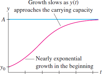
The simplest model of population growth is \({dy}/dt=ky\), according to which populations grow exponentially. This may be true over short periods of time, but it is clear that no population can increase without limit. Therefore, population biologists use a variety of other differential equations that take into account environmental limitations to growth such as food scarcity and competition between species. One widely used model is based on the logistic differential equation: \[ \begin{equation} \label{10.popmod.logsol} \boxed{\bbox[#FAF8ED,5pt]{\frac{dy}{dt} = ky \left(1-\frac{y}A \right),\qquad}}\tag {1} \end{equation} \] Here \(k>0\) is the growth constant, and \(A>0\) is a constant called the carrying capacity. Figure 9.19 shows a typical \(S\)-shaped solution of Eq. (1). As in the previous section, we also denote \({dy}/dt\) by \(\dot{y}\).
CONCEPTUAL INSIGHT
The logistic equation \(\dot{y} = ky(1 - y/A)\) differs from the exponential differential equation \(\dot{y}=ky\) only by the additional factor \((1-y/A)\). As long as \(y\) is small relative to \(A\), this factor is close to \(1\) and can be ignored, yielding \(\dot{y}\approx ky\). Thus, \(y(t)\) grows nearly exponentially when the population is small (Figure 9.19). As \(y(t)\) approaches \(A\), the factor \((1-y/A)\) tends to zero. This causes \(\dot{y}\) to decrease and prevents \(y(t)\) from exceeding the carrying capacity \(A\).
Solutions of the logistic equation with \(y_0<0\) are not relevant to populations because a population cannot be negative (see Exercise 18).
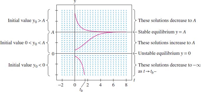
The slope field in Figure 9.20 shows clearly that there are three families of solutions, depending on the initial value \(y_0=y(0)\).
- If \(y_0>A\), then \(y(t)\) is decreasing and approaches \(A\) as \(t\to\infty\).
- If \(0< y_0<A\), then \(y(t)\) is increasing and approaches \(A\) as \(t\to\infty\).
- If \(y_0<0\), then \(y(t)\) is decreasing and \(\lim\limits_{t\to t_{b}-} y(t) = -\infty\) for some time \(t_b\).
Equation (1) also has two constant solutions: \(y=0\) and \(y=A\). They correspond to the roots of \(ky(1-y/A) = 0\), and they satisfy Eq. (1) because \(\dot{y}=0\) when \(y\) is a constant. Constant solutions are called equilibrium or steady-state solutions. The equilibrium solution \(y=A\) is a stable equilibrium because every solution with initial value \(y_0\) close to \(A\) approaches the equilibrium \(y=A\) as \(t\to \infty\). By contrast, \(y=0\) is an unstable equilibrium because every nonequilibrium solution with initial value \(y_0\) near \(y=0\) either increases to \(A\) or decreases to \(-\infty\).
525
In Eq. (2), we use the the partial fraction decomposition \[ \frac{1}{y \left(1-y/A \right)} = \frac{1}{y} - \frac{1}{y-A} \]
Having described the solutions qualitatively, let us now find the nonequilibrium solutions explicitly using separation of variables. Assuming that \(y\ne 0\) and \(y\ne A\), we have \[ \begin{align} \frac{dy}{dt} &= ky \left(1-\dfrac{y}A \right)\notag\\ \frac{dy}{y \left(1-y/A \right)} &= k\,dt\tag {2}\\ \int \left(\frac{1}{y} - \frac{1}{y-A}\right)dy &= \int k\, dt \label{10.popmod.partfrac}\notag\\ \ln |y| - \ln |y-A| &= kt+C\notag\\ \left|\frac{y}{y-A}\right| &=e^{kt+C} \quad\Rightarrow\quad \frac{y}{y-A} =\pm e^Ce^{kt}\notag \end{align} \] Since \(\pm e^{C}\) takes on arbitrary nonzero values, we replace \(\pm e^{C}\) with \(C\) (nonzero): \[ \begin{equation} \label{10.popmod.partlythere} \frac{y}{y-A} = Ce^{kt} \tag {3} \end{equation} \] For \(t=0\), this gives a useful relation between \(C\) and the initial value \(y_0=y(0)\): \[ \begin{equation} \label{10.popmod.loginit} \frac{y_0}{y_0-A} =C \tag {4} \end{equation} \] To solve for \(y\), multiply each side of Eq. (3) by \((y-A)\): \[ \begin{align*} y &= (y-A)Ce^{kt} \\ y(1-Ce^{kt}) &= - AC e^{kt}\\ y&= \frac{ AC e^{kt}}{ Ce^{kt}-1 } \end{align*} \] As \(C\ne 0\), we may divide by \(Ce^{kt}\) to obtain the general nonequilibrium solution: \[ \boxed{\bbox[#FAF8ED,5pt]{\frac{dy}{dt} = ky \left(1 - \frac{y}{A}\right),\qquad y= \frac{A}{1- e^{-kt}/C}}} \tag {5} \]
EXAMPLE 1
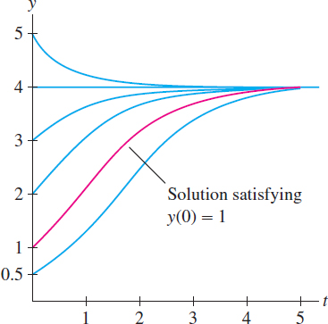
Solve \(\dot{y}=0.3y(4-y)\) with initial condition \(y(0)=1\).
Solution Recall that \(\dot{y} = \frac{dy}{dt}\). To apply Eq. (5), we must rewrite the equation in the form \[ \dot{y}=1.2y \left(1-\frac{y}4 \right) \] Thus, \(k=1.2\) and \(A=4\), and the general solution is \[ y= \frac{4}{1- e^{-1.2t}/C} \] There are two ways to find \(C\). One way is to solve \(y(0)=1\) for \(C\) directly. An easier way is to use Eq. (4): \[ C = \frac{y_0}{y_0-A} = \frac{1}{1-4}= -\frac13 \] We find that the particular solution is \(y= \frac{4}{1+3e^{-1.2t}}\) (Figure 9.21).
526
EXAMPLE 2 Deer Population
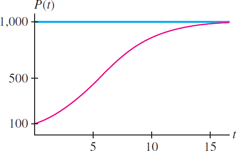
A deer population (Figure 9.22) grows logistically with growth constant \(k = 0.4 \mathrm{year}^{-1}\) in a forest with a carrying capacity of 1000 deer.
- Find the deer population \(P(t)\) if the initial population is \(P_0=100\).
- How long does it take for the deer population to reach 500?
The logistic equation may be too simple to describe a real deer population accurately, but it serves as a starting point for more sophisticated models used by ecologists, population biologists, and forestry professionals.
Solution The time unit is the year because the unit of \(k\) is \(\mathrm{year}^{-1}\).
- Since \(k=0.4\) and \(A=1000\), \(P(t)\) satisfies the differential equation \[ \frac{dP}{dt} = 0.4P \left(1-\frac{P}{1000}\right) \] The general solution is given by Eq. (5): \[ \begin{align} P(t) = \frac{1000}{1- e^{-0.4t}/C} \tag {6} \end{align} \] Using Eq. (4) to compute \(C\), we find (Figure 9.23) \[\begin{equation*} C = \frac{P_0}{P_0-A} = \frac{100}{100-1000}=-\frac19\quad\Rightarrow\quad P(t) = \frac{1000}{1+ 9e^{-0.4t}} \end{equation*}\]
- To find the time \(t\) when \(P(t)=500\), we could solve the equation \[ P(t) = \frac{1000}{1+ 9e^{-0.4t}} = 500 \] But it is easier to use Eq. (3): \begin{align*} \frac{P}{P-A}&=Ce^{kt}\\ \frac{P}{P-1000}&=-\frac19e^{0.4t} \end{align*} Set \(P=500\) and solve for \(t\): \[ -\dfrac19e^{0.4t} = \frac{500}{500-1000}=-1\quad\Rightarrow\quad e^{0.4t} =9 \quad\Rightarrow\quad 0.4t =\ln9 \] This gives \(t = (\ln 9)/0.4\approx 5.5\) years.
9.4.1 Summary
- The logistic equation and its general nonequilibrium solution (\(k>0\) and \(A>0\)): \[ \frac{dy}{dt} =ky\left(1-\frac{y}A\right),\qquad y= \frac{A}{1 - e^{-kt}/C}, \qquad\text{or equivalently}\qquad \frac{y}{y-A} = Ce^{kt} \]
- Two equilibrium (constant)solutions:
- - \(y=0\) is an unstable equilibrium.
- - \(y=A\) is a stable equilibrium.
- If the initial value \(y_0 = y(0)\) satisfies \(y_0 > 0\), then \(y(t)\) approaches the stable equilibrium \(y = A\); that is, \(\lim_{t\to\infty} y(t) = A\).
527