1.1 Vectors in Two- and Three-Dimensional Space
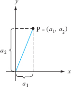
In this section we build our mathematical model of space. Points P in the plane are represented by ordered pairs of real numbers \((a_1,a_2)\); the numbers \(a_1\) and \(a_2\) are called the Cartesian coordinates of P. We draw two perpendicular lines, label them as the \(x\) and \(y\) axes, and then drop perpendiculars from P to these axes, as in Figure 1.1. After designating the intersection of the \(x\) and \(y\) axes as the origin and choosing units on these axes, we produce two signed distances \(a_1\) and \(a_2\) as shown in the figure; \(a_1\) is called the \(x\) component of P, and \(a_2\) is called the \(y\) component.
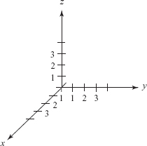
Points in space may be similarly represented as ordered triples of real numbers. To construct such a representation, we choose three mutually perpendicular lines that meet at a point in space. These lines are called \(x\) axis, \(y\) axis, and \(z\) axis, and the point at which they meet is called the origin (this is our reference point). We choose a scale on these axes, as shown in Figure 1.2.
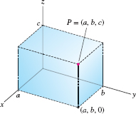
The triple (\(0,0,0\)) corresponds to the origin of the coordinate system, and the arrows on the axes indicate the positive directions. For example, if \(a,b\) and \(c\) are positive real numbers, then the triple (\(a, b, c\)) represents a point \(a\) units from the origin in the positive direction along the \(x\) axis, \(b\) units in the positive direction along the \(y\) axis, and \(c\) units in the positive direction along the \(z\) axis (Figure 1.3).
Because we can associate points in space with ordered triples in this way, we often use the expression “the point \((a_1,a_2,a_3)\)” instead of the longer phrase “the point P that corresponds to the triple \((a_1,a_2,a_3)\)” We say that \(a_1\) is the \(x\) coordinate (or first coordinate), \(a_2\) is the \(y\) coordinate (or second coordinate), and \(a_3\) is the \(z\) coordinate (or third coordinate) of P. It is also common to denote points in space with the letters \(x,y\), and \(z\) in place of \(a_1,a_2\), and \(a_3\). Thus, the triple \((x,y,z)\) represents a point whose first coordinate is \(x\), second coordinate is \(y\), and third coordinate is \(z\).
2
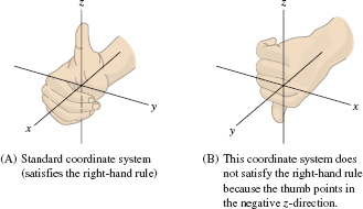
By convention, we label the axes as in Figure 1.4, where the positive sides of the axes are labeled \(x\), \(y\), and \(z\). This labeling satisfies the right-hand rule, which means that when you position your right hand so that your fingers curl from the positive \(x\)-axis toward the positive \(y\)-axis, your thumb points in the positive \(z\)-direction. The axes in Figure 1.4 are not labeled according to the right-hand rule.
We employ the following notation for the line, the plane, and three-dimensional space:
- (i) The real number line is denoted \({\mathbb R}^1\) or simply \({\mathbb R}\).
- (ii) The set of all ordered pairs \((x,y)\) of real numbers is denoted \({\mathbb R}^2\).
- (iii) The set of all ordered triples \((x,y,z)\) of real numbers is denoted \({\mathbb R}^3\).
When speaking of \({\mathbb R}^1,{\mathbb R}^2\), and \({\mathbb R}^3\) simultaneously, we write \({\mathbb R}^n\), where \(n=1,2\), or 3; or \({\mathbb R}^m\), where \(m=1,2,3\). Starting in Section 1.5 we will also study \({\mathbb R}^n\) for \(n=4,5,6,\ldots,\) but the cases \(n=1,2,3\) are closest to our geometric intuition and will be stressed throughout the book.
Addition and Scalar Multiplication of Ordered Pairs and Triples
The operation of addition can be extended from \({\mathbb R}\) to \({\mathbb R}^2\) and \({\mathbb R}^3\). For \({\mathbb R}^3\), this is done as follows. Given the two triples \((a_1,a_2,a_3)\) and \((b_1,b_2,b_3)\), we define their sum to be \[ (a_1,a_2,a_3)+(b_1,b_2,b_3)=(a_1+b_1,a_2+b_2,a_3+b_3). \]
3
example 1
\begin{eqnarray*} (1,1,1) + (2,-3,4) &=& (3,-2,5), \\ (x,y,z) + (0,0,0) &=& (x,y,z), \\ (1,7,3) + (a,b,c) & = & (1+a,7+b,3+c) \end{eqnarray*}
The element (\(0, 0, 0\)) is called the zero element (or just zero) of \({\mathbb R}^3\). The element \((-a_1,-a_2,-a_3)\) is the additive inverse (or negative) of \((a_1,a_2,a_3)\), and we will write \((a_1,\) \(a_2\), \(a_3)-(b_1,b_2,b_3)\) for \((a_1,a_2,a_3)+(-b_1,-b_2,-b_3)\).
The additive inverse, when added to the vector itself, of course produces zero: \[ (a_1, a_2, a_3) +(-a_1, -a_2, -a_3) =(0, 0, 0). \]
There are several important product operations that we will define on \({\mathbb R}^3\). One of these, called the inner product, assigns a real number to each pair of elements of \({\mathbb R}^3\). We shall discuss it in detail in Section 1.2. Another product operation for \({\mathbb R}^3\) is called scalar multiplication (the word “scalar” is a synonym for “real number”). This product combines scalars (real numbers) and elements of \({\mathbb R}^3\) (ordered triples) to yield elements of \({\mathbb R}^3\) as follows: Given a scalar \(\alpha\) and a triple \((a_1,a_2,a_3)\), we define the scalar multiple by \[ \alpha (a_1,a_2,a_3) = (\alpha a_1,\alpha a_2,\alpha a_3). \]
example 2
\begin{eqnarray*} 2(4,e,1) &=& (2\cdot 4, 2 \cdot e, 2 \cdot 1) = (8,2e,2), \\ 6 (1,1,1) &=& (6,6,6), \\ 1 (u,v,w) &=& (u,v,w),\\ 0 (\kern.5ptp,q,r) &=& (0, 0,0) \end{eqnarray*}
Question 1.1 Section 1.1 Progress Check Question 1
Find the sum of the tuple \((1,2,-2)\) and twice the tuple \((-2,3,5)\).
| A. |
| B. |
| C. |
| D. |
| E. |
Addition and scalar multiplication of triples satisfy the following properties:
- (i) \((\alpha\beta)(a_1, a_2, a_3) = \alpha[\beta(a_1, a_2, a_3)]\)(associativity)
- (ii) \((\alpha + \beta)(a_1, a_2, a_3) = \alpha(a_1, a_2, a_3) + \beta(a_1, a_2, a_3)\)(distributivity)
- (iii) \(\alpha[(a_1, a_2, a_3) + (b_1, b_2, b_3)] = \alpha(a_1, a_2, a_3) + \alpha(b_1, b_2, b_3)\)(distributivity)
- (iv) \(\alpha(0, 0, 0) = (0, 0, 0)\)(property of zero)
- (v) \(0(a_1, a_2, a_3) = (0, 0, 0)\)(property of zero)
- (vi) \(1(a_1, a_2, a_3) = (a_1, a_2, a_3)\)(property of the unit element)
The identities are proven directly from the definitions of addition and scalar multiplication. For instance, \begin{eqnarray*} (\alpha+\beta)(a_1,a_2,a_3) &=& ((\alpha+\beta)a_1,(\alpha+\beta)a_2, (\alpha+\beta)a_3)\\ &=& (\alpha a_1+\beta a_1, \alpha a_2+\beta a_2, \alpha a_3+\beta a_3)\\ &=& \alpha(a_1,a_2,a_3)+\beta(a_1,a_2,a_3). \end{eqnarray*}
For \({\mathbb R}^2\), addition and scalar multiplication are defined just as in \({\mathbb R}^3\), with the third component of each vector dropped off. All the properties (i) to (vi) still hold.
For example, \((1,1)+(2,3)=(3,4)\) and \(2(2,3)=(4,6)\). Also \((0,0)\) is the zero element of \({\mathbb R}^2\).
example 3
Interpret the chemical equation 2NH\(_2+{\rm H}_2=2\)NH\(_3\) as a relation in the algebra of ordered pairs.
solution We think of the molecule N\(_x\)H\(_y\) (\(x\) atoms of nitrogen, \(y\) atoms of hydrogen) as represented by the ordered pair \((x,y)\). Then the chemical equation given is equivalent to \(2(1,2)+(0,2)=2(1,3)\). Indeed, both sides are equal to (2, 6).
Geometry of Vector Operations
4
Let us turn to the geometry of these operations in \({\mathbb R}^2\) and \({\mathbb R}^3\). For the moment, we define a vector to be a directed line segment beginning at the origin; that is, a line segment with specified magnitude and direction, and initial point at the origin. Figure 1.5 shows several vectors, drawn as arrows beginning at the origin. In print, vectors are usually denoted by boldface letters such as \({\bf v}\) or \({\bf a}\). By hand, we usually write them as \(\vec{v}\) or simply as \(v\), possibly with a line or wavy line under it.
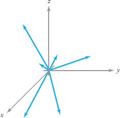
Using this definition of a vector, we associate with each vector \({\bf a}\) the point \((a_1,a_2,a_3)\) where \({\bf a}\) terminates, and conversely, we can associate a vector \({\bf v}\) with each point \((a_1,a_2,a_3)\) in space. Thus, we shall identify \({\bf a}\) with \((a_1,a_2,a_3)\) and write \({\bf a}=(a_1,a_2,a_3)\). For this reason, the elements of \({\mathbb R}^3\) not only are ordered triples of real numbers, but are also regarded as vectors. The triple (0, 0, 0) is denoted \({\bf 0}\). We call \(a_1,a_2\), and \(a_3\) the components of \({\bf a}\), or when we think of \({\bf a}\) as a point, its coordinates.
Two vectors \({\bf v}=(a_1,a_2,a_3)\) and \({\bf w}=(b_1,b_2,b_3)\) are equal if and only if \(a_1=b_1, a_2=b_2\), and \(a_3=b_3\). Geometrically this means that \({\bf v}\) and \({\bf w}\) have the same direction and the same length (or “magnitude”).
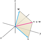
Geometrically, we define vector addition as follows. In the plane containing the vectors \({\bf v}=(a_1,a_2,a_3)\) and \({\bf w}=(b_1,b_2,b_3)\) (see Figure 1.6), form the parallelogram having \({\bf v}\) as one side and \({\bf w}\) as its adjacent side. The sum \({\bf v}+{\bf w}\) is the directed line segment along the diagonal of the parallelogram.
5
This geometric view of vector addition is useful in many physical situations, as we shall see in the next section. For an easily visualized example, consider a bird or an airplane flying through the air with velocity \({\bf v}_1\), but in the presence of a wind with velocity \({\bf v}_2\). The resultant velocity, \({\bf v}_1+{\bf v}_2,\) is what one sees; see Figure 1.7.

To show that our geometric definition of addition is consistent with our algebraic definition, we demonstrate that if \({\bf a}=(a_1, a_2, a_3)\) and \({\bf b}=(b_1, b_2, b_3)\), then \({\bf a}+{\bf b}=(a_1+b_1, a_2+b_2, a_3+b_3)\). We shall prove this result in the plane and leave the proof in three-dimensional space to the reader. Thus, we wish to show that if \({\bf a}=(a_1,a_2)\) and \({\bf b}=(b_1,b_2)\), then \({\bf a}+{\bf b}=(a_1+b_1,a_2+b_2)\).
In Figure 1.8 let \({\bf a}=(a_1,a_2)\) be the vector ending at the point A, and let \({\bf b}=(b_1,b_2)\) be the vector ending at point B. By definition, the vector \({\bf a}+{\bf b}\) ends at the vertex C of parallelogram OBCA. To verify that \({\bf a}+{\bf b}=(a_1+b_1,a_2+b_2)\), it suffices to show that the coordinates of C are \((a_1+b_1,a_2+b_2)\). The sides of the triangles OAD and BCG are parallel, and the sides OA and BC have equal lengths, which we write as OA \(=\) BC. These triangles are congruent, so BG \(=\) OD; since BGFE is a rectangle, EF \(=\) BG. Furthermore, OD \(=a_1\) and OE \(=b_1\). Hence, EF \(=\) BG \(=\) OD \(=a_1\). Since OF \(=\) EF \(+\) OE, it follows that OF \(=a_1+b_1\). This shows that the \(x\) coordinate of \({\bf a}+{\bf b}\) is \(a_1+b_1\). The proof that the \(y\) coordinate is \(a_2+b_2\) is analogous. This argument assumes A and B to be in the first quadrant, but similar arguments hold for the other quadrants.
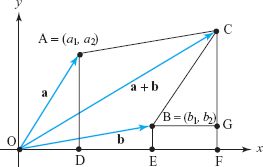
Figure 1.9 illustrates another way of looking at vector addition: in terms of triangles rather than parallelograms. That is, we translate (without rotation) the directed line segment representing the vector \({\bf b}\) so that it begins at the end of the vector \({\bf b}\). The endpoint of the resulting directed segment is the endpoint of the vector \({\bf a}+{\bf b}\). We note that when \({\bf a}\) and \({\bf b}\) are collinear, the triangle collapses to a line segment, as in Figure 1.9.
6
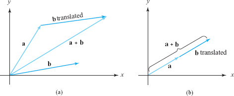
In Figure 1.9 we have placed \({\bf a}\) and \({\bf b}\) head to tail. That is, the tail of \({\bf b}\) is placed at the head of \({\bf a}\), and the vector \({\bf a}+{\bf b}\) goes from the tail of \({\bf a}\) to the head of \({\bf b}\). If we do it in the other order, \({\bf b}+{\bf a}\), we get the same vector by going around the parallelogram the other way. Consistent with this figure, it is useful to let vectors “glide” or “slide,” keeping the same magnitude and direction. We want, in fact, to regard two vectors as the same if they have the same magnitude and direction. When we insist on vectors beginning at the origin, we will say that we have bound vectors. If we allow vectors to begin at other points, we will speak of free vectors or just vectors.
Vectors
Vectors (also called free vectors) are directed line segments in [the plane or] space represented by directed line segments with a beginning (tail) and an end (head). Directed line segments obtained from each other by parallel translation (but not rotation) represent the same vector.
The components \((a_1,a_2,a_3)\) of \({\bf a}\) are the (signed) lengths of the projections of \({\bf a}\) along the three coordinate axes; equivalently, they are defined by placing the tail of\({\bf a}\) at the origin and letting the head be the point \((a_1,a_2,a_3)\). We write \({\bf a}\)=\((a_1,a_2,a_3)\).
Two vectors are added by placing them head to tail and drawing the vectors from the tail of the first to the head of the second, as in Figure 1.9.
Scalar multiplication of vectors also has a geometric interpretation. If \(\alpha\) is a scalar and \({\bf a}\) a vector, we define \(\alpha{\bf a}\) to be the vector that is \(|\alpha|\) times as long as \({\bf a}\), with the same direction as \({\bf a}\) if \(\alpha>0\), but with the opposite direction if \(\alpha<0\). Figure 1.10 illustrates several examples.

7
Using an argument based on similar triangles, we find that if \({\bf a}=(a_1,a_2,a_3)\), and \(\alpha\) is a scalar, then \[ \alpha \ {\bf a}=(\alpha a_1,\alpha a_2,\alpha a_3). \]
That is, the geometric definition coincides with the algebraic one.
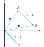
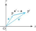
Given two vectors a and b, how do we represent the vector \({\bf b}-{\bf a}\) geometrically, that is, what is the geometry of vector subtraction? Because \({\bf a}+({\bf b}-{\bf a})={\bf b}\), we see that \({\bf b}-{\bf a}\) is the vector that we add to a to get b. In view of this, we may conclude that \({\bf b}-{\bf a}\) is the vector parallel to, and with the same magnitude as, the directed line segment beginning at the endpoint of a and terminating at the endpoint of b when a and b begin at the same point (see Figure 1.11).
example 4
Let u and v be the vectors shown in Figure 1.12. Draw the two vectors \({\bf u}+{\bf v}\) and \(-2{\bf u}\). What are their components?
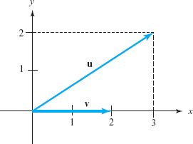
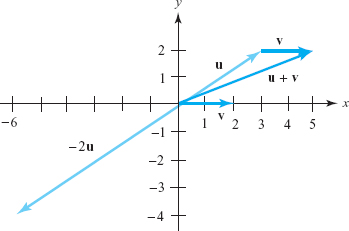
solution Place the tail of v at the tip of u to obtain the vector shown in Figure 1.13.
The vector \(-2{\bf u}\), also shown, has length twice that of u and points in the opposite direction. From the figure, we see that the vector \({\bf u}+{\bf v}\) has components (5, 2) and \(-2{\bf u}\) has components \((-6,-4)\).
8
example 5
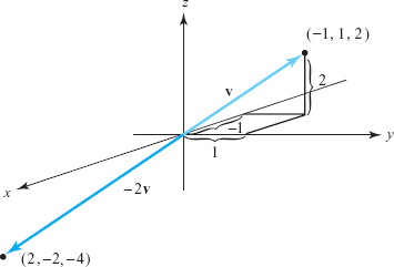
- (a) Sketch \(-2{\bf v}\), where \({\bf v}\) has components \((-1,1,2)\).
- (b) If \({\bf v}\) and \({\bf w}\) are any two vectors, show that \({\bf v}-\frac{1}{3}{\bf w}\) and \(3{\bf v}-{\bf w}\) are parallel.
solution
- (a) The vector \(-2{\bf v}\) is twice as long as \({\bf v}\), but points in the opposite direction (see Figure 1.14).
- (b) \({\bf v}-\frac{1}{3}{\bf w}=\frac{1}{3}(3{\bf v}-{\bf w})\); vectors that are multiples of one another are parallel.
The Standard Basis Vectors
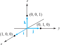
To describe vectors in space, it is convenient to introduce three special vectors along the \(x,y\), and \(z\) axes: \[ \begin{array}{c} {\bf i}{:}\, \hbox{ the vector with components (1, 0, 0)}\\ {\bf j}{:}\, \hbox{ the vector with components (0, 1, 0)}\\ {\bf k}{:}\, \hbox{ the vector with components (0, 0, 1)}. \end{array} \]
9
These standard basis vectors are illustrated in Figure 1.15. In the plane we have the standard basis \({\bf i}\) and \({\bf j}\) with components (1, 0) and (0, 1).
Let \({\bf a}\) be any vector, and let \((a_1,a_2,a_3)\) be its components. Then \[ {\bf a}=a_1{\bf i}+a_2{\bf j}+a_3{\bf k}, \] because the right-hand side is given in components by \begin{eqnarray*} a_1(1,0,0)+a_2(0,1,0)+a_3(0,0,1) &=& (a_1,0,0)+(0,a_2,0)+(0,0,a_3)\\ &=& (a_1,a_2,a_3). \end{eqnarray*}
Thus, we can express every vector as a sum of scalar multiples of \({\bf i},{\bf j}\), and \({\bf k}\).
The Standard Basis Vectors
- The vectors \({\bf i},{\bf j}\), and \({\bf k}\) are unit vectors along the three coordinate axes, as shown in Figure 1.15.
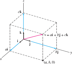
- If \({\bf v}\) has components \((a,b,c)\), then \[ {\bf v}=a{\bf i}+b{\bf j}+c{\bf k}. \] as shown in Figure 1.16.
example 6
Express the vector whose components are \((e,\pi,-\sqrt{3})\) in the standard basis.
solution Substituting \(a_1 = e, a_2=\pi,\) and \( a_3 = -\sqrt{3}\) into \({\bf a} = a_1 {\bf i} + a_2 {\bf j} + a_3 {\bf k}\) gives \[ {\bf v}=e{\bf i}+\pi{\bf j}-\sqrt{3}{\bf k}. \]
Question 1.2 Section 1.1 Progress Check Question 2
Express the vector whose components are \((-2, \frac12, 3) \) in the standard basis.
| A. |
| B. |
| C. |
| D. |
| E. |
example 7
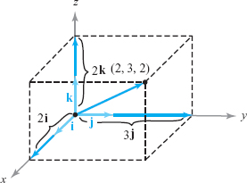
The vector (2, 3, 2) equals \(2{\bf i}+3{\bf j}+2{\bf k}\), and the vector \((0,-1,4)\) is \(-{\bf j} + 4{\bf k}\). Figure 1.17 shows \(2{\bf i}+3{\bf j}+2{\bf k}\); you draw in the vector \(-{\bf j}+4{\bf k}\).
Addition and scalar multiplication may be written in terms of the standard basis vectors as follows: \[ (a_1{\bf i}+a_2{\bf j}+a_3{\bf k})+(b_1{\bf i}+b_2{\bf j}+b_3{\bf k}) = (a_1+b_1){\bf i}+(a_2+b_2){\bf j}+(a_3+b_3){\bf k} \] and \[ \alpha(a_1{\bf i}+a_2{\bf j}+a_3{\bf k}) = (\alpha a_1){\bf i}+(\alpha a_2){\bf j}+\alpha(a_3){\bf k}. \]
10
The Vector Joining Two Points
To apply vectors to geometric problems, it is useful to assign a vector to a pair of points in the plane or in space, as follows. Given two points P and Q, we can draw the vector \({\bf v}\) with tail P and head Q, as in Figure 1.17, where we write \(\overrightarrow{{\rm PQ}}\) for \(\bf v\) .
If P \(=(x,y,z)\) and Q\(=(x',y',z')\), then the vectors from the origin to P and Q are \({\bf a}=\) \(x{\bf i}\) \(+\) \(y{\bf j}\) \(+\) \(z{\bf k}\) and \({\bf b}=x'{\bf i}+y'{\bf j}+z'{\bf k}\), respectively, so the vector \(\overrightarrow{{\rm PQ}}\) is the difference \({\bf b}-{\bf a}=(x'-x){\bf i}+(\kern1pty'-y){\bf j}+(z'-z){\bf k}\). (See Figure 1.19.).
The Vector Joining Two Points
If the point P has coordinates \((x,y,z)\) and Q has coordinates \((x',y',z')\), then the vector \(\overrightarrow{{\rm PQ}}\) from the tip of P to the tip of Q has components \((x'-x,y'-y,z'-z)\).
example 8
- (a) Find the components of the vector from (3, 5) to (4, 7).
- (b) Add the vector v from \((-1,0)\) to \((2,-3)\) and the vector w from (2, 0) to (1, 1).
- (c) Multiply the vector v in (b) by 8. If the resulting vector is represented by the directed line segment from (5, 6) to Q, what is Q?
solution
- (a) As in the preceding box, we subtract the ordered pairs: \((4, 7)-(3,5)=(1,2)\). Thus the required components are (1, 2).
- (b) The vector \({\bf v}\) has components \((2,-3)-(-1,0)=(3,-3)\), and w has components \((1,1)-(2,0)=(-1,1)\). Therefore, the vector \({\bf v}+{\bf w}\) has components \((3,-3)+ (-1,1) =\) \((2,-2)\).
- (c) The vector \(8{\bf v}\) has components \(8(3,-3)=(24,-24)\). If this vector is represented by the directed line segment from (5, 6) to Q, and Q has coordinates \((x,y)\), then \((x,y)-(5,6)=\) \((24,-24)\), so \((x,y)=(5,6)+(24,-24) = (29,-18)\).
Question 1.3 Section 1.1 Progress Check Question 3
Find the components of the vector \(\overrightarrow{\rm PQ}\) if P has coordinates \((-1,2,1)\) and Q has coordinates \((1,0,2)\).
| A. |
| B. |
| C. |
| D. |
example 9
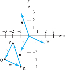
Let \({\rm P}=(-2,-1), {\rm Q}=(-3,-3)\), and \({\rm R}=(-1,-4)\) in the \(xy\) plane.
- (a) Draw these vectors: v joining P to Q; \({\bf w}\) joining Q to R; u joining R to P.
- (b) What are the components of \({\bf v},{\bf w}\), and \({\bf u}\)?
- (c) What is \({\bf v}+{\bf w}+{\bf u}\)?
11
solution
- (a) See Figure 1.20.
- (b) Because \({\bf v}= \overrightarrow{{\rm PQ}\vphantom{^\prime}}, {\bf w}= \overrightarrow{{\rm QR}\vphantom{^\prime}},\) and \({\bf u} = \overrightarrow{{\rm RP}\vphantom{^\prime}},\) we get \begin{eqnarray*} {\bf v} &=& (-3,-3)-(-2,-1)=(-1,-2),\\ {\bf w} &=& (-1,-4)-(-3,-3)=(2,-1),\\ {\bf u} &=& -(-1,-4)+(-2,-1)=(-1,3). \end{eqnarray*}
- (c) \({\bf v}+{\bf w}+ {\bf u} =(-1,-2)+(2,-1)+(-1,3)=(0,0)\).
Geometry Theorems by Vector Methods
Many of the theorems of plane geometry can be proved by vector methods. Here is one example.
example 10
Use vectors to prove that the diagonals of a parallelogram bisect each other.
solution Let OPRQ be the parallelogram, with two adjacent sides represented by the vectors \({\bf a}=\overrightarrow{\rm OP\vphantom{^\prime}}\) and \({\bf b}=\overrightarrow{\rm OQ\vphantom{^\prime}}\). Let M be the midpoint of the diagonal OR, and let N be the midpoint of the other diagonal, PQ. (See Figure 1.21.)

Observe that \(\overrightarrow{\rm OR\vphantom{^\prime}}=\overrightarrow{\rm OP\vphantom{^\prime}}+\overrightarrow{\rm OQ\vphantom{^\prime}}={\bf a}+{\bf b}\) by the parallelogram rule for vector addition, so \(\overrightarrow{\rm OM\vphantom{^\prime}}=\frac{1}{2}\overrightarrow{\rm OR\vphantom{^\prime}}=\frac{1}{2}\)(a+b). On the other hand, \[ \overrightarrow{\rm PQ\vphantom{^\prime}}=\overrightarrow{\rm OQ\vphantom{^\prime}}-\overrightarrow{\rm OP\vphantom{^\prime}}={\bf b}-{\bf a}, \qquad\hbox{so}\qquad \overrightarrow{\rm PN\vphantom{^\prime}} = {\textstyle \frac{1}{2}} \overrightarrow{\rm PQ\vphantom{^\prime}} = {\textstyle \frac{1}{2}} ({\bf b}-{\bf a}), \] and hence, \[ \overrightarrow{\rm ON\vphantom{^\prime}}=\overrightarrow{\rm OP\vphantom{^\prime}}+\overrightarrow{\rm PN\vphantom{^\prime}}=a+ {\textstyle \frac{1}{2}} (\bf{b-a}) = {\textstyle \frac{1}{2}}(\bf{a+b}). \]
12
Because \(\overrightarrow{\rm OM\vphantom{^\prime}}\) and \(\overrightarrow{\rm ON\vphantom{^\prime}}\) are equal vectors, the points M and N coincide, so the diagonals bisect each other.
Equations of Lines
Planes and lines are geometric objects that can be represented by equations. We shall defer until Section 1.3 a study of equations representing planes. However, using the geometric interpretation of vector addition and scalar multiplication, we will now find the equation of a line l that passes through the endpoint of the vector \({\bf a}\), with the direction of a vector \({\bf v}\) (see Figure 1.22); that is, line \(l\) is parallel to the vector v.
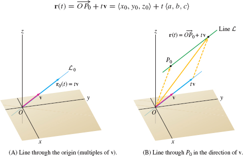
As \(t\) varies through all real values, the points of the form \(t{\bf v}\) are all scalar multiples of the vector v, and therefore exhaust the points of the line passing through the origin in the direction of v. Because every point on \(l\) is the endpoint of the diagonal of a parallelogram with sides a and \(t{\bf v}\) for some real value of \(t\), we see that all the points on \(l\) are of the form \({\bf a}+t{\bf v}\). Thus, the line \(l\) may be expressed by the equation \({\bf l}(t)={\bf a}+t{\bf v}\). We say that \(l\) is expressed parametrically, with \(t\) the parameter. At \(t=0,{\bf l}(t)={\bf a}\). As \(t\) increases, the point \({\bf l}(t)\) moves away from a in the direction of v. As \(t\) decreases from \(t=0\) through negative values, \({\bf l}(t)\) moves away from a in the direction of \(-{\bf v}\).
Point-Direction Form of a Line
The equation of the line \(l\) through the tip of a and pointing in the direction of the vector v is \({\bf l}(t)={\bf a}+ t{\bf v}\), where the parameter \(t\) takes on all real values. In coordinate form, the equations are \begin{eqnarray*} x &=& x_1+at,\\ y &=& y_1+bt,\\ z &=& z_1+ct, \end{eqnarray*} where \({\bf a}=(x_1,y_1,z_1)\) and \({\bf v}=(a,b,c)\). For lines in the \(xy\) plane, we simply drop the \(z\) component.
example 11
Determine the equation of the line \(l\) passing through (1, 0, 0) in the direction j. See Figure 1.23.
13
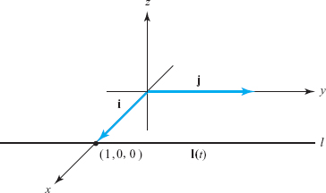
solution The desired line can be expressed parametrically as \({\bf l}(t)={\bf i}+t{\bf j}\). In terms of coordinates, \[ {\bf l}(t)=(1,0,0)+t(0,1,0)=(1,t,0). \]
example 12
- (a) Find the equations of the line in space through the point \((3,-1,2)\) in the direction \(2{\bf i}-3{\bf j}+4{\bf k}\).
- (b) Find the equation of the line in the plane through the point \((1,-6)\) in the direction of \(5{\bf i}-\pi{\bf j}\).
- (c) In what direction does the line \(x=-3t+2, y=-2(t-1), z=8t+2\) point?
solution
- (a) Here \({\bf a}=(3,-1,2)=(x_1,y_1,z_1)\) and \({\bf v}=2{\bf i}-3{\bf j}+4{\bf k}\), so \(a=2,b=-3\), and \(c=4\). From the preceding box, the equations are \[ x=3+2t,\qquad y=-1-3t,\qquad z=2+4t. \]
- (b) Here \({\bf a}=(1,-6)\) and \({\bf v}=5{\bf i}-\pi {\bf j}\), so the required line is \[ {\bf l}(t)=(1,-6)+(5t,-\pi t)=(1+5t,-6\,-\,\pi t); \] that is, \[ x=1+5t,\qquad y=-6\,-\,\pi t. \]
- (c) Using the box, we construct the direction \({\bf v}=a{\bf i}+b{\bf j}+c{\bf k}\) from the coefficients of \(t{:}\) \(a=-3,b=-2,c=8\). Thus, the line points in the direction of \({\bf v}=-3{\bf i}-2{\bf j}+8{\bf k}\).
Question 1.4 Section 1.1 Progress Check Question 4
Find an equation of the line in space through \((-1,2,0)\) in the direction of \({\bf v}= {\bf i}-{\bf j}+2 {\bf k}\)
| A. |
| B. |
| C. |
| D. |
example 13
Do the two lines \((x,y,z)=(t,-6t+1, 2t-8)\) and \((x,y,z)=\) \((3t+1,2t,0)\) intersect?
solution If the lines intersect, there must be numbers \(t_1\) and \(t_2\) such that the corresponding points are equal: \[ (t_1,-6t_1+1,2t_1-8) = (3t_2+1, 2t_2,0); \]
14
that is, all three of the following equations hold: \begin{eqnarray*} t_1 &=& 3t_2+1,\\ -6t_1+1 &=& 2t_2,\\ 2t_1-8 &=& 0. \end{eqnarray*}
From the third equation, \(t_1=4\). The first equation then becomes \(4=3t_2+1\); that is, \(t_2=1\). We must check whether these values satisfy the middle equation: \[ -6t_1+1 \stackrel{?}{=} 2t_2. \]
Since \(t_1=4\) and \(t_2=1\), this reads \[ -24+1 \stackrel{?}{=} 2, \] which is false, so the lines do not intersect.
There can be many equations of the same line. Some may be obtained by choosing, instead of \({\bf a}\), a different point on the given line, and forming the parametric equation of the line beginning at that point and in the direction of \({\bf v}\). For example, the endpoint of \({\bf a}+{\bf v}\) is on the line \({\bf l}(t)={\bf a}+t{\bf v}\), and thus, \({\bf l}_1(t)=({\bf a}+{\bf v})+t{\bf v}\) represents the same line. Still other equations may be obtained by observing that if \(\alpha \neq 0\), the vector \(\alpha {\bf v}\) has the same (or opposite) direction as \({\bf v}\). Thus, \({\bf l}_2(t)={\bf a}+t\alpha{\bf v}\) is another equation of \({\bf l}(t)={\bf a}+t{\bf v}\).
For example, both \({\bf l}(t)=(1,0,0)+(t,t,0)\) and \({\bf l}_1(s)=(0,-1,0)+(s,s,0)\) represent the same line since both are in the direction \({\bf i}+{\bf j}\) and both pass through the point (1, 0, 0); \({\bf l}\) passes through (1, 0, 0) at \(t=0\) and \({\bf l}_1\) passes through (1, 0, 0) at \(s=1\).
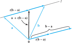
Therefore, the equation of a line is not uniquely determined. Nevertheless, it is customary to use the term “the equation of a line.” Keeping this in mind, let us derive the equation of a line passing through the endpoints of two given vectors \({\bf a}\) and \({\bf b}\). Because the vector \({\bf b}-{\bf a}\) is parallel to the directed line segment from \({\bf a}\) to \({\bf b}\), we calculate the parametric equation of the line passing through \({\bf a}\) in the direction of \({\bf b}-{\bf a}\) (Figure 1.24). Thus, \[ {\bf l}(t)={\bf a}+t({\bf b}-{\bf a});\qquad\hbox{that is},\qquad{\bf l}(t)=(1-t){\bf a}+t{\bf b}. \]
As \(t\) increases from 0 to 1, \(t({\bf b}-{\bf a})\) starts as the zero vector and increases in length (remaining in the direction of \({\bf b}-{\bf a}\)) until at \(t=1\) it is the vector \({\bf b}-{\bf a}\). Thus, for \({\bf l}(t)={\bf a}+t({\bf b}-{\bf a})\), as \(t\) increases from 0 to 1, the vector \({\bf l}(t)\) moves from the endpoint of \({\bf a}\) to the endpoint of \({\bf b}\) along the directed line segment from \({\bf a}\)to \({\bf b}\).
Question 1.5 Section 1.1 Progress Check Question 5
Which of the following three equations represent the same line?
\({\bf l_1}(t) = (1,1,2)+ t(1,2,3)\)
\({\bf l_2}(t) = (2,2,4)+ t(2,4,6)\)
\({\bf l_3}(t) = (1,1,2)+ t(2,4,6)\)
| A. |
| B. |
| C. |
| D. |
| E. |
15
If P \(=(x_1,y_1,z_1)\) is the tip of \({\bf a}\) and Q \(=(x_2,y_2,z_2)\) is the tip of \({\bf b}\), then \({\bf v} = (x_2-x_1){\bf i} + (\kern1pty_2-y_1){\bf j} + (z_2-z_1){\bf k}\), and so the equations of the line are \begin{eqnarray*} x &=& x_1 +(x_2-x_1)t,\\ y &=& y_1+(\kern1pty_2-y_1)t,\\ z &=& z_1+(z_2-z_1)t.\\[-21pt] \end{eqnarray*}
By eliminating \(t\), these can be written as \[ \frac{x-x_1}{x_2-x_1}=\frac{y-y_1}{y_2-y_1}=\frac{z-z_1}{z_2-z_1}. \]
Parametric Equation of a Line: Point-Point Form
The parametric equations of the line \(l\) through the points \({\rm P}=(x_1,y_1,z_1)\) and \({\rm Q} =(x_2,y_2,z_2)\) are \begin{eqnarray*} x &=& x_1+(x_2-x_1)t,\\ y &=& y_1+(\kern1pty_2-y_1)t,\\ z &=& z_1+(z_2-z_1)t, \end{eqnarray*} where \((x,y,z)\) is the general point of \(l\), and the parameter \(t\) takes on all real values.
example 14
Find the equation of the line through \((2,1,-3)\) and \((6,-1,-5)\).
solution Using the preceding box, we choose \((x_1,y_1,z_1)=(2,1,-3)\) and \((x_2, y_2\), \(z_2)\) \(=\) \((6,-1,-5)\), so the equations are \begin{eqnarray*} x &=& 2+(6-2)t=2+4t,\\ y &=& 1+(-1-1)t=1-2t,\\ z &=& -3+(-5-(-3))t=-3-2t.\\[-36pt] \end{eqnarray*}
example 15
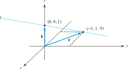
Find the equation of the line passing through \((-1,1,0)\) and (0, 0, 1) (see Figure 1.25).
16
solution Letting \({\bf a}=-{\bf i}+{\bf j}\) and \({\bf b}={\bf k}\) represent the given points, we have \[ {\bf l}(t)=(1-t)(-{\bf i}+{\bf j})+t{\bf k}=-(1-t){\bf i}+(1-t){\bf j}+t{\bf k}. \] The equation of this line may thus be written as \[ {\bf l}(t)=(t-1){\bf i}+(1-t){\bf j}+t{\bf k}, \] or, equivalently, if \({\bf l}(t)=x{\bf i}+y{\bf j}+z{\bf k}\), \[ x=t-1,\qquad\hskip-3pty=1-t,\qquad\hskip-3ptz=t. \]
The description of a line segment requires that the domain of the parameter \(t\) be restricted, as in the following example.
example 16
Find the equation of the line segment between (1, 1, 1) and (\(2, 1, 2\)).
solution The line through (1, 1, 1) and (2, 1, 2) is described in parametric form by \((x,y,z)=(1+t,1,1+t)\), as \(t\) takes on all real values. When \(t=0\), the point \((x,y,z)\) is (1, 1, 1), and when \(t=1\), the point \((x,y,z)\) is (2, 1, 2). Thus, the point \((x,y,z)\) lies between (1, 1, 1) and (2, 1, 2) when \(0\leq t\leq 1\), so the line segment is described by the equations \begin{eqnarray*} x &=& 1+t,\\ y &=& 1,\\ z &=& 1+t, \end{eqnarray*} together with the inequalities \(0\leq t\leq 1\).
We can also give parametric descriptions of geometric objects other than lines.
example 17
Describe the points that lie within the parallelogram whose adjacent sides are the vectors \({\bf a}\) and \({\bf b}\) based at the origin (“within” includes points on the edges of the parallelogram).
solution Consider Figure 1.26. If P is any point within the given parallelogram and we construct lines \(l_1\) and \(l_2\) through P parallel to the vectors \({\bf a}\) and \({\bf b}\), respectively, we see that \(l_1\) intersects the side of the parallelogram determined by the vector b at some point \(t{\bf b}\), where \(0\leq t\leq 1\). Likewise, \(l_2\) intersects the side determined by the vector \({\bf a}\) at some point \(s{\bf a}\), where \(0\leq s\leq 1\).
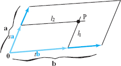
Note that P is the endpoint of the diagonal of a parallelogram having adjacent sides \(s{\bf a}\) and \(t{\bf b}\); hence, if \({\bf v}\) denotes the vector \(\overrightarrow{\rm OP\vphantom{^\prime}}\), we see that \({\bf v}=s{\bf a}+t{\bf b}\). We conclude that all the points in the given parallelogram are endpoints of vectors of the form \(s{\bf a}+t{\bf b}\) for \(0\leq s\leq 1\) and \(0\leq t\leq 1\). Reversing our steps, we see that all vectors of this form end within the parallelogram.
17
As two different lines through the origin determine a plane through the origin, so do two nonparallel vectors. If we apply the same reasoning as in Example 17, we see that the entire plane formed by two nonparallel vectors \({\bf v}\) and \({\bf w}\) consists of all points of the form \(s{\bf v}+t{\bf w}\), where \(s\) and \(t\) can be any real numbers, as in Figure 1.27.
We have thus described the points in the plane by two parameters. For this reason, we say the plane is two-dimensional. Similarly, a line is called one-dimensional whether it lies in the plane or in space or is the real number line itself.
The plane determined by \({\bf v}\) and \({\bf w}\) is called the plane spanned by \({\bf v}\) and \({\bf w}\). When \({\bf v}\) is a scalar multiple of \({\bf w}\) and \({\bf w}\neq {\bf 0}\), then v and \({\bf w}\) are parallel and the plane degenerates to a straight line. When \({\bf v}={\bf w}={\bf 0}\) (i.e., both are zero vectors), we obtain a single point.
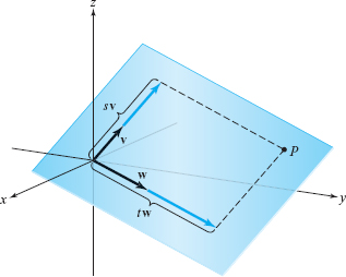
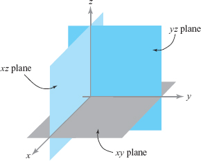
There are three particular planes that arise naturally in a coordinate system and that will be useful to us later. We call the plane spanned by vectors \({\bf i}\) and \({\bf j}\) the \(xy\) plane, the plane spanned by \({\bf j}\) and \({\bf k}\) the \(yz\) plane, and the plane spanned by \({\bf i}\) and \({\bf k}\) the \(xz\) plane. These planes are illustrated in Figure 1.28.
