11.7 \(n\)-Dimensional Euclidean Space
Vectors in \(n\)-space
In Sections 1.1 and 1.2 we studied the spaces \({\mathbb R} = {\mathbb R}^1, {\mathbb R}^2\), and \({\mathbb R}^3\) and gave geometric interpretations to them. For example, a point \((x,y,z)\) in \({\mathbb R}^3\) can be thought of as a geometric object, namely, the directed line segment or vector emanating from the origin and ending at the point \((x,y,z)\). We can therefore think of \({\mathbb R}^3\) in either of two ways:
- (i) Algebraically, as a set of triples \((x,y,z)\), where \(x,y,\) and \(z\) are real numbers
- (ii) Geometrically, as a set of directed line segments
These two ways of looking at \({\mathbb R}^3\) are equivalent. For generalization it is easier to use definition (i). Specifically, we can define \({\mathbb R}^n\), where \(n\) is a positive integer (possibly greater than 3), to be the set of all ordered \(n\)-tuples \((x_1, x_2, \ldots, x_n)\), where the \(x_i\) are real numbers. For instance, \((1, \sqrt{5},2, \sqrt{3}) \in {\mathbb R}^4\).
The set \({\mathbb R}^n\) so defined is known as euclidean n-space, and its elements, which we write as \({\bf x} = (x_1,x_2, \ldots,\) \(x_n)\), are known as vectors or n-vectors. By setting \(n=1,2\), or 3, we recover the line, the plane, and three-dimensional space, respectively.
Having the notion of euclidean \(n\)-space at our disposal will allow us to consider all the myriad of vector valued functions all at once, rather than one at a time. It will also provide us with a general definition of "the derivative'' of a vector valued function of several variables, a definition which took several hundred years to discover. Such abstract reasoning helps us to smplify and consolidate mathematics.
We launch our study of euclidean \(n\)-space by introducing several algebraic operations. These are analogous to those introduced in Section 11.1 for \({\mathbb R}^2\) and \({\mathbb R}^3\). The first two, addition and scalar multiplication, are defined as follows:
- (i) \((x_1, x_2, \ldots , x_n) + ( y_1, y_2, \ldots, y_n) = (x_1 + y_1, x_2 + y_2, \ldots , x_n + y_n)\); and
- (ii) for any real number \(\alpha\), \[ \alpha (x_1, x_2, \ldots, x_n) = (\alpha x_1,\alpha x_2, \ldots ,\alpha x_n). \]
The geometric significance of these operations for \({\mathbb R}^2\) and \({\mathbb R}^3\) was discussed in Section 11.1.
The \(n\) vectors \[ {\bf e}_1 =(1,0,0, \ldots , 0), {\bf e}_2 = (0,1,0, \ldots , 0), \ldots , {\bf e}_n\,{=}\, (0,0, \ldots , 0,1) \] are called the standard basis vectors of \({\mathbb R}^n\), and they generalize the three mutually orthogonal unit vectors \({\bf i,j,k}\) of \({\mathbb R}^3\). The vector \({\bf x} = (x_1, x_2, \ldots , x_n)\) can then be written as \({{\bf x} =x_1 {\bf e}_1 + x_2 {\bf e}_2 + \cdots + x_n {\bf e}_n}\).
For two vectors \({\bf x} = (x_1, x_2, x_3)\) and \({\bf y}= (\kern1pty_1, y_2, y_3)\) in \({\mathbb R}^3\), we defined the dot or inner product \({\bf x \,{\cdot}\, y}\) to be the real number \({\bf x \,{\cdot}\, y} = x_1 y_1 + x_2 y_2 + x_3 y_3\). This definition easily extends to \({\mathbb R}^n\); specifically, for \({\bf x} = ( x_1, x_2, \ldots ,x_n) , {\bf y} = (y_1, y_2, \ldots , y_n)\), we define the inner product of \({\bf x}\) and \({\bf y}\) to be \({\bf x \,{\cdot}\, y} = x_1 y_1 + x_2 y_2 + \cdots + x_n y_n\). In \({\mathbb R}^n\), the notation \(\langle {\bf x, y} \rangle\) is often used in place of \({\bf x \,{\cdot}\, y}\) for the inner product.
Continuing the analogy with \({\mathbb R}^3\), we are led to define the notion of the length or norm of a vector \({\bf x}\) by the formula \[ \hbox{Length of } {\bf x} = \|{\bf x} \| =\textstyle\sqrt{ {\bf x} \ {\cdot}\ {\bf x}} =\sqrt{x_1^2 + x_2^2 + \cdots + x_n^2}. \]
If x and y are two vectors in the plane \(({\mathbb R}^2)\) or in space \(({\mathbb R}^3)\), then we know that the angle \(\theta\) between them is given by the formula \[ \cos \theta = \frac{ {\bf x \,{\cdot}\, y}}{\|{\bf x}\|\|{\bf y}\|}. \]
61
The right side of this equation can be defined in \({\mathbb R}^n\) as well as in \({\mathbb R}^2\) or \({\mathbb R}^3\). It still represents the cosine of the angle between x and y; this angle is geometrically well defined, because x and y lie in a two-dimensional subspace of \({\mathbb R}^n\) (the plane determined by x and y) and our usual geometry ideas apply to such planes.
It will be useful to have available some algebraic properties of the inner product. These are summarized in the next theorem [compare with properties (i), (ii), (iii), and (iv) of Section 11.2].
Theorem 3
For \({\bf x,y,z} \in {\mathbb R}^n\) and \(\alpha, \beta,\) real numbers, we have
- (i) \(( \alpha {\bf x} + \beta {\bf y} ) \,{\cdot}\, {\bf z} = \alpha ( {\bf x \,{\cdot}\, z}) + \beta ( {\bf y \,{\cdot}\, z})\).
- (ii) \({\bf x \,{\cdot}\, y} = {\bf y \,{\cdot}\, x}.\)
- (iii) \({\bf x \,{\cdot}\, x} \ge 0.\)
- (iv) \({\bf x \,{\cdot}\, x} =0\) if and only if \({\bf x} ={\bf 0}.\)
proof
Each of the four assertions can be proved by a simple computation. For example, to prove property (i) we write \begin{eqnarray*} ( \alpha {\bf x} + \beta {\bf y}) \,{\cdot}\, {\bf z} & = & ( \alpha x_1 + \beta y_1 , \alpha x_2 + \beta y_2 , \ldots , \alpha x_n + \beta y_n ) \,{\cdot}\, (z_1, z_2 , \ldots , z_n ) \\ & = & ( \alpha x_1 + \beta y_1) z_1 + ( \alpha x_2 + \beta y_2 ) z_2 + \cdots + (\alpha x_n + \beta y_n) z_n \\ & = & a x_1 z_1 + \beta y_1 z_1 + \alpha x_2 z_2 + \beta y_2 z_2 + \cdots + \alpha x_nz_n + \beta y_n z_n \\ & = & \alpha ( {\bf x \,{\cdot}\, z}) + \beta ( {\bf y \,{\cdot}\, z}). \end{eqnarray*}
The other proofs are similar.
In Section 11.2, we proved an interesting property of dot products, called the Cauchy–Schwarz inequality.4 For \({\mathbb R}^2\) our proof required the use of the law of cosines. For \({\mathbb R}^n\) we could also use this method, by confining our attention to a plane in \({\mathbb R}^n\). However, we can also give a direct, completely algebraic proof.
Theorem 4 Cauchy-Schwarz Inequality in \({\mathbb R}^{n}\)
Let \({\bf x}, {\bf y}\) be vectors in \({\mathbb R}^n\). Then \[ |{\bf x} \,{\cdot}\, {\bf y} | \le \| {\bf x}\| \|{\bf y}\|. \]
proof
Let \(a = {\bf y \,{\cdot}\, y}\) and \(b = - {\bf x \,{\cdot}\, y}.\) If \(a=0\), the theorem is clearly valid, because then \({\bf y} ={\bf 0}\) and both sides of the inequality reduce to 0. Thus, we may suppose \(a \ne 0\).
62
By Theorem 3 we have \begin{eqnarray*} 0 \le ( a {\bf x} + b {\bf y}) \,{\cdot}\, (a {\bf x} + b {\bf y}) & = & a^2 {\bf x \,{\cdot}\, x} +2 ab {\bf x \,{\cdot}\, y} + b^2 {\bf y \,{\cdot}\, y} \\ & = & ( {\bf y \,{\cdot}\, y} )^2 {\bf x \,{\cdot}\, x} - ( {\bf y \,{\cdot}\, y}) ( {\bf x \,{\cdot}\, y})^2.\\ \end{eqnarray*}
Dividing by \({\bf y \,{\cdot}\, y}\) gives \(0 \le ( {\bf y \,{\cdot}\, y} ) ( {\bf x \,{\cdot}\, x}) - ( {\bf x \,{\cdot}\, y})^2\), that is, \(( {\bf x \,{\cdot}\, y})^2 \le ( {\bf x \,{\cdot}\, x}) ( {\bf y \,{\cdot}\, y}) = \| {\bf x} \|^2 \| {\bf y} \|^2\). Taking square roots on both sides of this inequality yields the desired result.
There is a useful consequence of the Cauchy–Schwarz inequality in terms of lengths. The triangle inequality is geometrically clear in \({\mathbb R}^3\) and was discussed in Section 11.2. The analytic proof of the triangle inequality that we gave in Section 11.2 works exactly the same in \({\mathbb R}^n\) and proves the following:
Corollary Triangle Inequality in \({\mathbb R}^n\)
Let \({\bf x},{\bf y}\) be vectors in \({\mathbb R}^n\). Then \[ \|{\bf x}+{\bf y}\|\leq \|{\bf x}\|+\|{\bf y}\|. \]
If Theorem 4 and its corollary are written out algebraically, they become the following useful inequalities: \begin{eqnarray*} &\displaystyle \left| \sum_{i=1}^n x_i y_i \right| \le \left( \sum_{i=1}^n x_i^2 \right)^{1/2} \left( \sum_{i=1}^n y_i^2 \right)^{1/2}; \\[6pt] & \displaystyle \left( \sum_{i=1}^n ( x_i + y_i)^2 \right)^{1/2} \le \left( \sum_{i=1}^n x_i^2 \right)^{1/2} + \left( \sum_{i=1}^n y_i^2 \right)^{1/2}. \end{eqnarray*}
example 1
Let \({\bf x} = (1,2,0,-1)\) and \({\bf y} = (-1,1,1,0)\). Verify Theorem 4 and its corollary in this case.
solution
\begin{eqnarray*} \\[-30pt] \|{\bf x}\| & = & \sqrt{1^2 + 2^2 + 0^2 + (-1)^2} = \sqrt{6} \\[3pt] \|{\bf y}\| & = & \sqrt{(-1)^2 + 1^2 + 1^2 + 0^2} = \sqrt{3} \\[3pt] {\bf x \,{\cdot}\, y} & = & 1 \cdot (-1) + 2 \,{\cdot}\, 1 + 0 \,{\cdot}\, 1 + (-1) \cdot 0 =1 \\[3pt] {\bf x} + {\bf y} & = & (0,3,1,-1) \\[3pt] \|{\bf x} + {\bf y} \| & = & \sqrt{ 0^2 + 3^2 + 1^2 + (-1)^2} = \sqrt{11}. \end{eqnarray*}
We compute \({\bf x \,{\cdot}\, y} =1 \le 4.24 \approx \sqrt{6} \sqrt{3} = \|{\bf x} \|\|{\bf y}\|\), which verifies Theorem 4. Similarly, we can check its corollary: \begin{eqnarray*} \|{\bf x} + {\bf y} \| & = & \sqrt{11} \approx 3.32 \\ &\le& 4.18 = 2.45 + 1.73 \approx \sqrt{6} + \sqrt{3} = \|{\bf x}\| + \|{\bf y} \|. \\ \end{eqnarray*}
By analogy with \({\mathbb R}^3\), we can define the notion of distance in \({\mathbb R}^n\); namely, if \({\bf x}\) and \({\bf y}\) are points in \({\mathbb R}^n\), the distance between \({\bf x}\) and \({\bf y}\) and \({\bf y}\) is defined to be \(\|{\bf x} - {\bf y} \|\), or the length of the vector \({\bf x} - {\bf y}\). We do not attempt to define the cross product on \({\mathbb R}^n\) except for \(n=3\).
Question 11.175 Section 11.7 Progress Check Question 1
Find the distance between \( {\bf x} \) and \( \bf{y} \) where \( {\bf{x}} = (1,\dfrac{1}{2}, 2, -1,-2, 0) \) and \( {\bf{y}} = (0,1, 0, -2,1, \dfrac{\sqrt{3}}{2}) \)
| A. |
| B. |
| C. |
| D. |
| E. |
63
General Matrices
Generalizing \(2 \times 2 \) and \(3 \times 3\) matrices (see Section 11.3), we can consider \(m \times n\) matrices, which are arrays of \(mn\) numbers: \[ A = \left[ \begin{array}{@{}c@{\hskip9pt}c@{\hskip9pt}c@{\hskip9pt}c@{}} a_{11} & a_{12} & \cdots & a_{1n} \\ a_{21} & a_{22} & \cdots & a_{2n} \\ \vdots & \vdots & & \vdots \\ a_{m1} & a_{m2} & \cdots & a_{mn} \end{array} \right]\!. \]
We shall also write \(A\) as \([a_ij]\). We define addition and multiplication by a scalar componentwise, just as we did for vectors. Given two \(m \times n\) matrices \(A\) and \(B\), we can add them to obtain a new \(m \times n\) matrix \(C= A+B \), whose \(ij\,\)th entry \(c_ij\) is the sum of \(a_ij\) and \(b_ij\). It is clear that \(A+B = B + A\).
example 2
(a) \(\bigg[\begin{array}{@{}c@{\quad}c@{\quad}c@{}} 2 & 1 & 0 \\ 3 & 4 & 1 \end{array}\bigg] + \bigg[\begin{array}{@{}r@{\quad}c@{\quad}c@{}} -1 & 1 & 3\\ 0 & 0 & 7 \end{array}\bigg] = \bigg[\begin{array}{@{}c@{\quad}c@{\quad}c@{}} 1 & 2 & 3 \\ 3 & 4 & 8 \end{array}\bigg]\).
(b) \([1{\quad}2] + [0{\quad}-1]= [ 1{\quad}1].\)
(c) \(\left[ \begin{array}{cc} 2 & 1\\ 1 & 2 \end{array}\right] - \left[\begin{array}{cc}1 & 0 \\ 0 & 1 \end{array}\right] = \bigg[\begin{array}{cc} 1 & 1 \\ 1 & 1 \end{array}\bigg].\)
Given a scalar \(\lambda\) and an \(m \times n\) matrix \(A\), we can multiply \(A\) by \(\lambda\) to obtain a new \(m \times n\) matrix \(\lambda A =C\), whose \(ij\,\)th entry \(c_{ij}\) is the product \(\lambda a_{ij}\).
example 3
\[ 3 \ \left[\begin{array}{@{}c@{\quad}r@{\quad}c@{}} 1 & -1 & 2 \\ 0 & 1 & 5 \\ 1 & 0 & 3 \end{array}\right] = \left[\begin{array}{@{}c@{\quad}r@{\quad}r@{}} 3 & -3 & 6 \\ 0 & 3 & 15 \\ 3 & 0 & 9 \end{array}\right]\!. \]
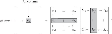
Next we turn to matrix multiplication. If \(A = [a_{ij}], B = [b_{ij} ]\) are \(n \times n\) matrices, then the product \(AB=C\) has entries given by \[ c_{ij} = \sum_{k=1}^n a_{ik} b_{kj}, \] which is the dot product of the \(i\)th row of \(A\) and the \(j\)th column of \(B\):
64
example 4
Let \[ A= \left[\begin{array}{@{}c@{\quad}c@{\quad}c@{}} 1 & 0 & 3 \\ 2 & 1 & 0 \\ 1 & 0 & 0 \end{array} \right] \ \ \ \ \ {\rm and} \qquad B = \left[\begin{array}{@{}c@{\quad}c@{\quad}c@{}} 0 & 1 & 0 \\ 1 & 0 & 0 \\ 0 & 1 & 1 \end{array} \right]\!. \]
Then \[ AB = \left[\begin{array}{@{}c@{\quad}c@{\quad}c@{}} 0 & 4 & 3 \\ 1 & 2 & 0 \\ 0 & 1 & 0 \end{array} \right] \ \ \ \ \ {\rm and} \qquad BA = \left[\begin{array}{@{}c@{\quad}c@{\quad}c@{}} 2 & 1 & 0 \\ 1 & 0 & 3 \\ 3 &1 & 0 \end{array} \right]\!. \]
Observe that \(AB\neq BA\).
Similarly, we can multiply an \(m \times n\) matrix (\(m\) rows, \(n\) columns) by an \(n \times p\) matrix (\(n\) rows, \(p\) columns) to obtain an \(m \times p\) matrix (\(m\) rows, \(p\) columns) by the same rule. Note that for \(AB\) to be defined, the number of columns of \(A\) must equal the number of rows of \(B\).
example 5
Let \[ A = \left[\begin{array}{@{}c@{\quad}c@{\quad}c@{}} 2 & 0 & 1 \\ 1 & 1 & 2 \end{array} \right] \ \ \ \ \ {\rm and} \qquad B = \left[\begin{array}{@{}c@{\quad}c@{\quad}c@{}} 1 & 0 & 2 \\ 0 & 2 & 1 \\ 1 & 1 & 1 \end{array} \right]\!. \] Then \[ AB= \left[\begin{array}{@{}c@{\quad}c@{\quad}c@{}} 3 & 1 & 5 \\ 3 & 4 & 5 \end{array} \right]\!, \] and \(BA\) is not defined.
Question 11.176 Section 11.7 Progress Check Question 2
Let \( A=\left[ \begin{array}{@{}c@{\quad}c@{\quad}c@{\quad}c@{}} 1 & 3 & 2 & -2 \\ -2 & 0 & 1 & 0 \end{array} \right] \) and \( B=\left[ \begin{array}{c} 1 \\ 0 \\ 1 \\ 2 \end{array} \right]\).
Find \(AB\).
| A. |
| B. |
| C. |
| D. |
| E. |
example 6
Let \[ A = \left[ \begin{array}{@{}c@{}} 1 \\ 2\\ 1\\ 3 \end{array} \right] \ \ \ \ \ {\rm and} \qquad B = [2 \quad 2 \quad 1 \quad 2]. \] Then \[ AB = \left[\begin{array}{@{}c@{\quad}c@{\quad}c@{\quad}c@{}} 2 & 2 & 1 & 2 \\ 4 & 4 & 2 & 4 \\ 2 & 2 & 1 & 2 \\ 6 & 6 & 3 & 6 \end{array} \right] \ \ \ \ \ {\rm and} \qquad BA = [13]. \]
Any \(m\,\times \, n\) matrix \(A\) determines a mapping of \({\mathbb R}^n\) to \({\mathbb R}^m\) defined as follows: Let \({\bf x} = (x_1, \ldots ,\) \(x_n) \in {\mathbb R}^n\); consider the \(n \,\times \,1\) column matrix associated with \({\bf x}\), which we shall temporarily denote \({\bf x}^T\) \[ {\bf x}^T = \left[\begin{array}{c} x_1 \\ \vdots \\ x_n \end{array} \right], \]
65
and multiply \(A\) by \({\bf x}^T\) (considered to be an \(n \times 1\) matrix) to get a new \(m \times 1\) matrix: \[ A {\bf x}^T = \left[\begin{array}{@{}c@{\quad}c@{\quad}c@{}} a_{11} & \cdots & a_{1n} \\ \vdots & & \vdots \\ a_{m1} & \cdots & a_{mn} \end{array} \right] \left[\begin{array}{@{}c@{}} x_1 \\ \vdots \\ x_n \end{array} \right] = \left[\begin{array}{@{}c@{}} y_1 \\ \vdots \\ y_m \end{array} \right] = {\bf y}^T, \]
corresponding to the vector \({\bf y} = (y_1, \ldots , y_m)\).5 Thus, although it may cause some confusion, we will write \({\bf x} = (x_1 , \ldots, x_n)\) and \({\bf y} =(\kern1pty_1, \ldots , y_m)\) as column matrices \[ {\bf x} = \left[ \begin{array}{@{}c@{}} x_1 \\ \vdots \\ x_n \end{array} \right]\!, {\bf y} = \left[ \begin{array}{@{}c@{}} y_1 \\ \vdots \\ y_m \end{array} \right] \]
when dealing with matrix multiplication; that is, we will identify these two forms of writing vectors. Thus, we will delete the \(T\) on \({\bf x}^T\) and view \({\bf x}^T\) and x as the same.
Thus, \(A{\bf x} ={\bf y}\) will “really” mean the following: Write x as a column matrix, multiply it by \(A\), and let y be the vector whose components are those of the resulting column matrix. The rule \({\bf x} \mapsto A {\bf x}\) therefore defines a mapping of \({\mathbb R}^n\) to \({\mathbb R}^m\). This mapping is linear; that is, it satisfies \begin{eqnarray*} & A( {\bf x} + {\bf y}) = A {\bf x} + A {\bf y} \\ & A ( \alpha {\bf x}) = \alpha ( A {\bf x}), \alpha \hbox{ a scalar}, \end{eqnarray*} as may be easily verified. One learns in a linear algebra course that, conversely, any linear transformation of \({\mathbb R}^n\) to \({\mathbb R}^m\) is representable in this way by an \(m \times n\) matrix.
If \(A =[a_{ij}]\) is an \(m \times n\) matrix and \({\bf e}_j\) is the \(j\)th standard basis vector of \({\mathbb R}^n\), then \(A {\bf e}_j\) is a vector in \({\mathbb R}^m\) with components the same as the \(j\)th column of \(A\). That is, the \(i\)th component of \(A {\bf e}_j\) is \(a_{ij}\). In symbols, \((A {\bf e}_j)_i = a_{ij}\).
example 7
If \[ A = \left[\begin{array}{@{}r@{\quad}c@{\quad}c@{}} 1 & 0 & 3 \\ -1 & 0 & 1\\ 2 & 1 & 2 \\ -1 & 2 & 1 \end{array} \right]\!, \] then \({\bf x} \mapsto A {\bf x}\) of \({\mathbb R}^3\) to \({\mathbb R}^4\) is the mapping defined by \[ \left[\begin{array}{c} x_1 \\ x_2 \\ x_3 \end{array} \right] \mapsto \left[\begin{array}{c} x_1 + 3 x_3 \\ -x_1 + x_3 \\ 2 x_1 + x_2 + 2 x_3 \\ -x_1 + 2 x_2 + x_3 \end{array} \right]\!. \]
66
example 8
The following illustrates what happens to a specific point when mapped by a \(4 \times 3\) matrix\(:\) \[ A {\bf e}_2 = \left[\begin{array}{@{}c@{\quad}c@{\quad}c@{}} 4 & 2 & 9 \\ 3 & 5 & 4 \\ 1 & 2 & 3 \\ 0 & 1 & 2 \end{array} \right] \left[\begin{array}{c} 0 \\ 1\\ 0 \end{array} \right] = \left[\begin{array}{c} 2 \\ 5 \\ 2\\ 1 \end{array} \right] = {\rm 2nd \ column\ of\ } A. \]
Properties of Matrices
Matrix multiplication is not, in general, commutative: If \(A\) and \(B\) are \(n \times n\) matrices, then generally \[ AB \ne BA, \] as Examples 4, 5, and 6 show.
An \(n \times n\) matrix is said to be invertible if there is an \(n \times n\) matrix \(B\) such that \[ AB =BA = I_n, \] where \[ I_n = \left[\begin{array}{@{}c@{\quad}c@{\quad}c@{\quad}c@{\quad}c@{}} \\ 1 & 0 & 0 & \cdots & 0 \\[1pt] 0 & 1 & 0 & \cdots & 0 \\[1pt] 0 & 0 & 1 & \cdots & 0 \\[1pt] \vdots & \vdots & \vdots & & \vdots \\[1pt] 0 & 0 & 0 & \cdots & 1 \end{array} \right] \] is the \(n \times n\) identity matrix: \(I_n\) has the property that \(I_n C = C I_n =C\) for any \(n \times n\) matrix \(C\). We denote \(B\) by \(A^{-1}\) and call \(A^{-1}\) the inverse of \(A\). The inverse, when it exists, is unique.
example 9
If \[ A = \left[\begin{array}{@{}c@{\quad}c@{\quad}c@{}} 2 & 4 & 0 \\ 0 & 2 & 1 \\ 3 & 0 & 2 \end{array} \right]\!, {\rm then} \qquad A^{-1} = \frac{1}{20} \left[\begin{array}{@{}r@{\quad}r@{\quad}r@{}} 4 & -8 & 4 \\ 3 & 4 & -2 \\ -6 & 12 & 4 \end{array} \right]\!, \] because \(AA^{-1} = I_3 = A^{-1} A,\) as may be checked by matrix multiplication.
Methods of computing inverses are learned in linear algebra; we won’t require these methods in this book. If \(A\) is invertible, the equation \(A {\bf x} = {\bf y}\) can be solved for the vector x by multiplying both sides by \(A^{-1}\) to obtain \({\bf x} = A^{-1} {\bf y}\).
In Section 11.3 we defined the determinant of a \(3 \times 3\) matrix. This can be generalized by induction to \(n \times n\) determinants. We illustrate here how to write the determinant of a \(4 \times 4\) matrix in terms of the determinants of \(3 \times 3\) matrices: \begin{eqnarray*} \left|\begin{array}{@{}c@{\quad}c@{\quad}c@{\quad}c@{}} a_{11} & a_{12} & a_{13} & a_{14} \\[1pt] a_{21} & a_{22} & a_{23} & a_{24} \\[1pt] a_{31} & a_{32} & a_{33} & a_{34} \\[1pt] a_{41} & a_{42} & a_{43} & a_{44} \end{array} \right| & = & a_{11}\left|\begin{array}{@{}c@{\quad}c@{\quad}c@{}} a_{22} & a_{23} & a_{24} \\[1pt] a_{32} & a_{33} & a_{34} \\[1pt] a_{42} & a_{43} & a_{44} \end{array} \right| -a_{12} \left|\begin{array}{@{}c@{\quad}c@{\quad}c@{}} a_{21} & a_{23} & a_{24} \\[1pt] a_{31} & a_{33} & a_{34} \\[1pt] a_{41} & a_{43} & a_{44} \end{array} \right| \\ && + \, a_{13} \left|\begin{array}{@{}c@{\quad}c@{\quad}c@{}} a_{21} & a_{22} & a_{24} \\[1pt] a_{31} & a_{32} & a_{34} \\[1pt] a_{41} & a_{42} & a_{44} \end{array} \right| - a_{14} \left| \begin{array}{@{}c@{\quad}c@{\quad}c@{}} a_{21} & a_{22} & a_{23} \\[1pt] a_{31} & a_{32} & a_{33} \\[1pt] a_{41} & a_{42} & a_{43} \end{array} \right| \\[-12pt] \end{eqnarray*} [see formula (2) of Section 11.3; the signs alternate \(+, -, +, -\)].
67
The basic properties of \(3 \times 3\) determinants reviewed in Section 11.3 remain valid for \(n \times n\) determinants. In particular, we note the fact that if \(A\) is an \(n \times n\) matrix and \(B\) is the matrix formed by adding a scalar multiple of one row (or column) of \(A\) to another row (or, respectively, column) of \(A\), then the determinant of \(A\) is equal to the determinant of \(B\) (see Example 10).
A basic theorem of linear algebra states that an \(n \times n\) matrix \(A\) is invertible if and only if the determinant of \(A\) is not zero. Another basic property is that the determinant is multiplicative: \(\hbox{det } (AB) = (\hbox{det } A) (\hbox{det } B)\). In this text, we shall not make use of many details of linear algebra, and so we shall leave these assertions unproved.
example 10
Let \[ A=\left[ \begin{array}{@{}c@{\quad}c@{\quad}c@{\quad}c@{}} 1 & 0 & 1 & 0 \\ 1 & 1 & 1 & 1 \\ 2 & 1 & 0 & 1 \\ 1 & 1 & 0 & 2 \end{array} \right]. \]
Find det A. Does A have an inverse?
solution Adding \((-1)\times \hbox{first}\) column to the third column, we get \[ \hbox{det } A = \left|\begin{array}{@{}c@{\quad}c@{\quad}r@{\quad}c@{}} 1 & 0 & 0 & 0 \\ 1 & 1 & 0 & 1 \\ 2 & 1 & -2 & 1 \\ 1 & 1 & -1 & 2 \end{array} \right| =1 \left|\begin{array}{@{}c@{\quad}r@{\quad}c@{}} 1 & 0 & 1 \\ 1 & -2 & 1 \\ 1 & -1 & 2 \end{array} \right| . \]
Adding \((-1) \times \hbox{first}\) column to the third column of this \(3 \times 3\) determinant gives \[ \hbox{det } A = \left|\begin{array}{@{}c@{\quad}r@{\quad}c@{}} 1 & 0 & 0 \\ 1 & -2 & 0 \\ 1 & -1 & 1 \end{array} \right| = \left|\begin{array}{cc} -2 & 0 \\ -1 & 1 \end{array} \right| = -2. \]
Thus, \(\hbox{det } A = -2 \ne 0\), and so \(A\) has an inverse.
Question 11.177 Section 11.7 Progress Check Question 3
Let \[ A=\left[ \begin{array}{@{}c@{\quad}c@{\quad}c@{\quad}c@{}} 1 & -1 & 2 & 1 \\ 7 & -1 & 3 & 0 \\ 2 & -2 & 4 & 2 \\ 1 & 1 & -5 & 2 \end{array} \right]. \] Find det (\(A\)). Hint: Think about this before you start calculating.
If we have three matrices \(A, B\), and \(C\) such that the products \(AB\) and \(BC\) are defined, then the products \((AB)C\) and \(A(BC)\) are defined and are in fact equal (i.e., matrix multiplication is associative). We call this the triple product of matrices and denote it by \(ABC\).
68
example 11
Let \[ A = \left[\begin{array}{c} 3 \\ 5 \end{array} \right], B = [ 1\quad 1], \hbox{and} \qquad C = \left[\begin{array}{c} 1 \\ 2 \end{array} \right]. \]
Then \[ ABC = A(BC) = \left[\begin{array}{c} 3 \\ 5 \end{array} \right] [3] = \left[\begin{array}{c} 9 \\ 15 \end{array} \right]. \]
example 12
\[ \left[\begin{array} &2 & 0 \\ 0 & 1 \end{array} \right] \left[\begin{array} &1 & 1 \\ 1 & 1 \end{array} \right] \left[\begin{array}{@{}c@{\quad}r@{}} 0 & -1 \\ 1 & 1 \end{array} \right] = \left[\begin{array} &2 & 0 \\ 0 & 1 \end{array} \right] \left[\begin{array} &1 & 0 \\ 1 & 0 \end{array} \right] = \left[\begin{array} &2 & 0 \\ 1 & 0 \end{array} \right] \]
Historical Note
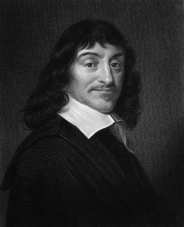
The founder of modern (coordinate) geometry was René Descartes (see Figure 11.117), a great physicist, philosopher, and mathematician, as well as a founder of modern biology.
Born in Touraine, France, in 1596, Descartes had a fascinating life. After studying law, he settled in Paris, where he developed an interest in mathematics. In 1628, he moved to Holland, where he wrote his only mathematical work, La Geometrie, one of the origins of modern coordinate geometry.
Descartes had been highly critical of the geometry of the ancient Greeks, with all their undefined terms and with their proofs requiring ever newer and more ingenious approaches. For Descartes, this geometry was so tied to geometric figures “that it can exercise the understanding only on condition of greatly fatiguing the imagination.” He undertook to exploit, in geometry, the use of algebra, which had recently been developed. The result was La Geometrie, which made possible analytic or computational methods in geometry.
Remember that the Greeks were, like Descartes, philosophers as well as mathematicians and physicists. Their answer to the question of the meaning of space was “Euclidean geometry.” Descartes had therefore succeeded in “algebrizing” the Greek model of space.
Gottfried Wilhelm Leibniz, cofounder (with Isaac Newton) of calculus, was also interested in “space analysis,” but he did not think that Descartes’s algebra went far enough. Leibniz called for a direct method of space analysis (analysis situs) that could be interpreted as a call for the development of vector analysis.
On September 8, 1679, Leibniz outlined his ideas in a letter to Christian Huygens:
I am still not satisfied with algebra, because it does not give the shortest methods or the most beautiful constructions in geometry. This is why I believe that, so far as geometry is concerned, we need still another analysis which is distinctly geometrical or linear and which will express situation (situs) directly as algebra expresses magnitude directly. And I believe that I have found the way and that we can represent figures and even machines and movements by characters, as algebra represents numbers or magnitudes. I am sending you an essay which seems to me to be important.
In the essay, Leibniz described his ideas in greater detail.