12.1 Paths and Curves
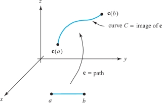
We often think of a curve as a line drawn on paper, such as a straight line, a circle, or a sine curve. It is useful to think of a curve \(C\) mathematically as the set of values of a function that maps an interval of real numbers into the plane or space. We shall call such a map a path. We usually denote a path by \({\bf c}\). The image \(C\) of the path then corresponds to the curve we see on paper (see Figure 12.1). Often we write t for the independent variable and imagine it to be time, so that \({\bf c}(t)\) is the position at time t of a moving particle, which traces out a curve as \(t\) varies. We also say c parametrizes \(C\). Strictly speaking, we should distinguish between \({\bf c}(t)\) as a point in space and as a vector based at the origin.
117
example 1
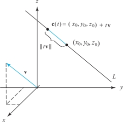
The straight line \(L\) in \({\mathbb R}^3\) through the point \((x_0,y_0,z_0)\) in the direction of vector \({\bf v}\) is the image of the path \[ {\bf c}(t)=(x_0,y_0,z_0)+t{\bf v} \] for \(t\in {\mathbb R}\) (see Figure 12.3). Thus, our notion of curve includes straight lines as special cases.
example 2
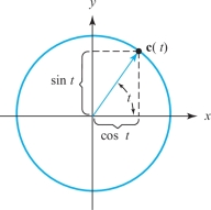
The unit circle \(C\): \(x^2+y^2=1\) in the plane is the image of the path \[ {\bf c}\,\colon\,{\mathbb R}\to{\mathbb R}^2, {\bf c}(t)=(\cos t,\sin t), 0\leq t\leq 2\pi \] (see Figure 12.4). The unit circle is also the image of the path \(\tilde{\bf c} (t)=(\cos 2t,\sin 2t)\), \(0\leq t\leq \pi\). Thus, different paths may parametrize the same curve.
Paths and Curves
A path in \({\mathbb R}^n\) is a map \({\bf c}\,{:}\,\,[a,b]\to{\mathbb R}^n\); it is a path in the plane if \(n=2\) and a path in space if \(n=3\). The collection \(C\) of points \({\bf c}(t)\) as \(t\) varies in \([a,b]\) is called a curve, and \({\bf c}(a)\) and \({\bf c}(b)\) are its endpoints. The path c is said to parametrize the curve \(C\). We also say \({\bf c}(t)\) traces out \(C\) as \(t\) varies.
If \({\bf c}\) is a path in \({\mathbb R}^3\), we can write \({\bf c}(t)=(x(t),y(t),z(t))\), and we call \(x(t),y(t)\), and \(z(t)\) the component functions of \({\bf c}\). We form component functions similarly in \({\mathbb R}^2\) or, generally, in \({\mathbb R}^n\). We also consider paths whose domain is the whole real line as in the next example.
example 3
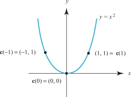
The path \({\bf c}(t)=(t,t^2)\) traces out a parabolic arc. This curve coincides with the graph \(f(x)=x^2\) (see Figure 12.5).
118
Question 12.1 Section 12.1 Progress Check Question 1
What planar curve is traced out by the path \({\bf c}(t) = ( 4 \cos (2t), 4 \sin (2t))\)?
| A. |
| B. |
| C. |
| D. |
| E. |
example 4
A wheel of radius \(R\) rolls to the right along a straight line at speed \(v\). Using vector method,we can find the path \({\bf c}(t)\) of the point on the wheel that initially lies at a distance \(r\) below the center.
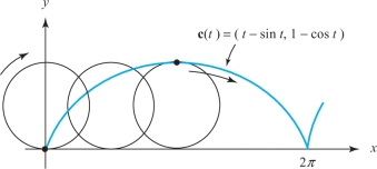
The formula for \({\bf c}(t)\) is given by \[ {\bf c}(t)=\bigg(vt-r\sin\frac{vt}{R}, R-r\cos\frac{vt}{R}\bigg). \]
In the special case \(v=R=r=1\), we get \({\bf c}(t)=(t-\sin t,1-\cos t)\). The image curve \(C\) of this path c is shown in Figure 12.6; it is called a cycloid.
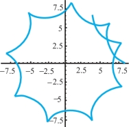
The preceding example considered the path of a point not necessarily on the rim of a wheel rolling along a straight line. When the wheel rolls on a circle, the resulting curve is called an epicycle. These are the epicycles discussed in the Ptolemaic theory in the introduction. If the wheel is outside the circle and the point is on the rim, the curve is called an epicycloid, and when the wheel is inside the circle, it is a hypocycloid. An example of the latter is shown in Figure 12.7.
Historical Note
The French mathematician Blaise Pascal studied the cycloid in 1649 as a way of distracting himself at a time when he was suffering from a painful toothache. When the pain disappeared, he took it as a sign that God was not displeased with his thoughts. Pascal’s results stimulated other mathematicians to investigate this curve, and subsequently numerous remarkable properties were found. One of these was discovered by the Dutchman Christian Huygens, who used it in the construction of a “perfect” pendulum clock.
A curve in \({\bf R}^3\) is also referred to as a space curve (as opposed to a curve in \({\bf R}^2\), which is called a plane curve or planar curve). Space curves can be quite complicated and difficult to sketch by hand. The most effective way to visualize a space curve is to plot it from different viewpoints using a computer (Figure 12.8). As an aid to visualization, we plot a “thickened” curve as in Figure 12.8 and Figure 12.10, but keep in mind that space curves are one-dimensional and have no thickness.

The projections onto the coordinate planes are another aid in visualizing space curves. The projection of a path \({\bf c}(t)=( x(t), y(t), z(t))\) onto the \(xy\)-plane is the path \({\bf p}(t) = ( x(t), y(t), 0)\) (Figure 12.9). Similarly, the projections onto the \(yz\)- and \(xz\)-planes are the paths \(( 0, y(t), z(t))\) and \(( x(t), 0, z(t))\), respectively.
725
EXAMPLE 5 Helix
Describe the curve traced by \({\bf c}(t) = ( {-\sin t}, \cos t, t)\) for \(t \geq 0\) in terms of its projections onto the coordinate planes.
Solution The projections are as follows (Figure 12.9):
- \(xy\)-plane (set \(z=0\)): the path \({\bf p}(t)=( {-\sin t}, \cos t,0)\), which describes a point moving counterclockwise around the unit circle starting at \({\bf p}(0) = (0,1,0)\).
- \(xz\)-plane (set \(y=0\)): the path \(( {-\sin t}, 0, t)\), which is a wave in the \(z\)-direction.
- \(yz\)-plane (set \(x=0\)): the path \(( 0, \cos t, t)\), which is a wave in the \(z\)-direction.
The function \({\bf c}(t)\) describes a point moving above the unit circle in the \(xy\)-plane while its height \(z=t\) increases linearly, resulting in the helix of Figure 12.9 .

Every curve can be parametrized in infinitely many ways (because there are infinitely many ways that a point can traverse a curve as a function of time). The next example describes two very different parametrizations of the same curve.
EXAMPLE 6 Parametrizing the Intersection of Surfaces
Parametrize the curve \(C\) obtained as the intersection of the surfaces \(x^2-y^2 = z-1\) and \(x^2+y^2=4\) (Figure 12.10).
Solution We have to express the coordinates \((x,y,z)\) of a point on the curve as functions of a parameter \(t\). Here are two ways of doing this.
First method: Solve the given equations for \(y\) and \(z\) in terms of \(x\). First, solve for \(y\): \[ x^2+y^2=4\quad\Rightarrow\quad y^2 = 4-x^2\quad\Rightarrow\quad y = \pm \sqrt{4-x^2} \]
The equation \(x^2-y^2=z-1\) can be written \(z=x^2-y^2+1\). Thus, we can substitute \(y^2 = 4-x^2\) to solve for \(z\): \[ z = x^2-y^2+1 = x^2 - (4-x^2)+1 = 2x^2-3 \]
726

Now use \(t=x\) as the parameter. Then \(y = \pm\sqrt{4-t^2}\), \(z =2t^2-3\). The two signs of the square root correspond to the two halves of the curve where \(y>0\) and \(y<0\), as shown in Figure 12.11. Therefore, we need two vector-valued functions to parametrize the entire curve: \[ {\bf c}_1(t) = ( t, \sqrt{4-t^2}, 2t^2-3),\quad {\bf c}_2(t) = ( t, -\sqrt{4-t^2}, 2t^2-3),\qquad -2\le t \le 2 \]

Second method: Note that \(x^2+y^2=4\) has a trigonometric parametrization: \(x = 2\cos t\), \(y = 2\sin t\) for \(0 \le t < 2\pi\). The equation \(x^2-y^2 = z-1\) gives us \[ z = x^2-y^2+1 = 4\cos^2t-4\sin^2t+1=4\cos 2t +1 \]
Thus, we may parametrize the entire curve by a single vector-valued function: \[ {\bf c}(t) = ( 2\cos t, 2\sin t, 4\cos 2t +1), \qquad \textrm{ \(0 \le t < 2\pi\)} \]
The Calculus of Paths
The first step is to define limits of paths.
DEFINITION Limit of a Path
A path \({\bf c}(t)\) approaches the limit \({\bf u}\) (a vector) as \(t\) approaches \(t_0\) if \(\displaystyle{\lim_{t\to t_0}\|{{\bf c}(t)-{\bf u}}\|={\bf 0}}\). In this case, we write \[ \lim_{t\to t_0}{\bf c}(t) = {\bf u} \]
We can visualize the limit of a vector-valued function as a vector \({\bf c}(t)\) “moving” toward the limit vector \({\bf u}\) (Figure 12.12). According to the next theorem, vector limits may be computed componentwise.

THEOREM 1 Limits Are Computed Componentwise
A path \({\bf c}(t)=( x(t), y(t), z(t))\) approaches a limit as \(t\to t_0\) if and only if each component approaches a limit, and in this case, \[ \lim_{t\to t_0}{\bf c}(t) = ( \lim_{t\to t_0}x(t), \lim_{t\to t_0}y(t), \lim_{t\to t_0}z(t))\tag{1} \]
Proof
Let \({\bf u} = ( a,b,c)\) and consider the square of the length \[ \|{{\bf c}(t)-{\bf u}}\|^2 = (x(t)-a)^2+(y(t)-b)^2+(z(t)-c)^2\tag{2} \]
The term on the left approaches zero if and only if each term on the right approaches zero (because these terms are nonnegative). It follows that \(\|{{\bf c}(t)-{\bf u}}\|\) approaches zero if and only if \(|x(t)-a|\), \(|y(t)-b|\), and \(|z(t)-c|\) tend to zero. Therefore, \({\bf c}(t)\) approaches a limit \({\bf u}\) as \(t\to t_0\) if and only if \(x(t)\), \(y(t)\), and \(z(t)\) converge to the components \(a\), \(b\), and \(c\).
Note
The Limit Laws of scalar functions remain valid in the vector-valued case. They are verified by applying the Limit Laws to the components.
EXAMPLE 1
Calculate \(\displaystyle{\lim_{t\to 3}{\bf c}(t)}\), where \(\displaystyle{{\bf c}(t) = ( t^2, 1-t, t^{-1})}\).
Solution By Theorem 1, \[ \lim_{t\to 3}{\bf c}(t) = \lim_{t\to 3}( t^2, 1-t, t^{-1}) = ( \lim_{t\to 3}t^2, \lim_{t\to 3}(1-t), \lim_{t\to 3} t^{-1}) = ( 9, -2, \frac13) \]
732
Continuity of vector-valued functions is defined in the same way as in the scalar case. A path \({\bf c}(t)=( x(t), y(t), z(t))\) is continuous at \(t_0\) if \[ \lim_{t\to t_0}\,{\bf c}(t) = {\bf c}(t_0) \]
By Theorem 1, \({\bf c}(t)\) is continuous at \(t_0\) if and only if the components \(x(t)\), \(y(t)\), \(z(t)\) are continuous at \(t_0\).
We say that \({\bf c}(t)\) is differentiable at \(t\) if the limit
\[ \boxed{\bbox[#FAF8ED,5pt]{{\bf c}'(t) = \dfrac{d}{dt}{\bf c}(t) = \lim\limits_{h\to 0} \frac{{\bf c}(t+h) - {\bf c}(t)}{h}}} \]
exists.
By Theorem 1, \({\bf c}(t)\) is differentiable if and only if the components are differentiable. In this case, \({\bf c}'(t)\) is equal to the vector of derivatives \(( x'(t), y'(t), z'(t))\).
Question 12.2 Section 12.1 Progress Check Question 2
Find the derivative of \({\bf c}(t) = (t^3, t^2, t)\).
| A. |
| B. |
| C. |
| D. |
Velocity and Tangents to Paths
If we think of \({\bf c}(t)\) as the curve traced out by a particle and \(t\) as time, it is reasonable to define the velocity vector as follows.
120
Definition: Velocity Vector
If \({\bf c}\) is a path and it is differentiable, we say \({\bf c}\) is a differentiable path. The velocity of c at time \(t\) is defined by \[ {{\bf c}'(t)=\mathop{\rm lim}_{h\to 0} \frac{{\bf c}(t+h)-{\bf c}(t)}{h}.} \]
We normally draw the vector \({\bf c}'(t)\) with its tail at the point \({\bf c}(t)\). The speed of the path \({\bf c}(t)\) is \(s=\|{\bf c}'(t)\|\), the length of the velocity vector. If \({\bf c}(t)=(x(t),y(t))\) in \({\mathbb R}^2\), then \[ {\bf c}'(t)=(x'(t),y'(t))=x'(t){\bf i}+y'(t){\bf j} \] and if \({\bf c}(t)=(x(t),y(t),z(t))\) in \({\mathbb R}^3\), then \[ {\bf c}'(t)=(x'(t),y'(t),z'(t))=x'(t){\bf i}+y'(t){\bf j}+z'(t){\bf k}. \]
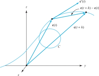
Here, \(x'(t)\) is the one-variable derivative \(dx/dt\). If we accept limits of vectors interpreted componentwise, the formulas for the velocity vector follow from the definition of the derivative. However, the limit can be interpreted in the sense of vectors as well. In Figure 12.13, we see that \([{\bf c}(t+h)-{\bf c}(t)]/h\) approaches the tangent to the path as \(h\to 0\).
Tangent Vector
The velocity \({\bf c}'(t)\) is a vector tangent to the path \({\bf c}(t)\) at time \(t\). If \(C\) is a curve traced out by c and if \({\bf c}'\)(\(t\)) is not equal to 0, then \({\bf c}'(t)\) is a vector tangent to the curve \(C\) at the point \({\bf c}(t)\).
121
example 5
Compute the tangent vector to the path \({\bf c}(t)=(t,t^2,e^t)\) at \(t=0\).
solution Here \({\bf c}'(t)=(1,2t,e^t)\), and so at \(t=0\) we obtain the tangent vector \((1, 0, 1)\).
example 6
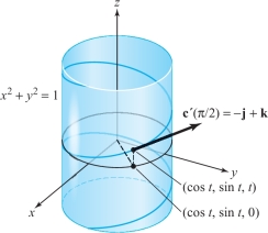
Describe the path \({\bf c}(t)=(\cos t,\sin t,t)\). Find the velocity vector at the point on the image curve where \(t=\pi/2\).
solution For a given \(t\), the point \((\cos t, \sin t, 0)\) lies on the circle \(x^2+y^2\,{=}\,1\) in the \(xy\) plane. Therefore, the point \((\cos t,\sin t, t)\) lies \(t\) units above the point \((\cos t, \sin t, 0)\) if \(t\) is positive and \(-t\) units below \((\cos t,\sin t,0)\) if \(t\) is negative. As \(t\) increases, \((\cos t,\sin t, t)\) wraps around the cylinder \(x^2+y^2=1\) with the z coordinate increasing. The curve this traces out is called a helix, which is depicted in Figure 12.14. At \(t=\pi/2,{\bf c}'(\pi/2)=({-}{\rm sin}\,\pi/2,\cos \pi/2,1)=(-1,0,1)=-{\bf i}+{\bf k}\).
example 7
The cycloidal path of a particle on the edge of a wheel of radius \(R\) with speed \(v\) is given by \({\bf c}(t)=(vt-R\sin\, (vt/R), R-R\cos \,(vt/R))\). (See Example 4.) Find the velocity \({\bf c}'(t)\) of the particle as a function of \(t\). When is the velocity zero? Is the velocity vector ever vertical?
solution To find the velocity, we differentiate: \begin{eqnarray*} {\bf c}'(t) &=& \bigg(\frac{d}{dt}\,\bigg(vt-R\sin\frac{vt}{R}\bigg), \frac{d}{dt}\,\bigg(R-R\cos\frac{vt}{R}\bigg)\bigg)\\[5.3pt] &=& \bigg(v-v\cos\frac{vt}{R},v\sin\frac{vt}{R}\bigg). \end{eqnarray*}
In vector notation, \({\bf c}'(t)=(v-v\cos\, (vt/R)){\bf i}+(v\sin\, (vt/R)){\bf j}\). The component in the direction of \({\bf i}\) is \(v(1-\cos\, (vt/R))\), which is zero whenever \(vt/R\) is an integer multiple of \(2\pi\). For such values of \(t\), \(\sin \,(vt/R)\) is zero as well, so the only times at which the velocity is zero are when \(t=2\pi{n}R/v\) for some integer \(n\). At such times, \({\bf c}(t)=(2\pi{n}R, 0)\), so the moving point is touching the ground. These moments occur at time intervals of \(2\pi\!R/v\) (more frequently for small wheels, as well as for rapidly rolling ones).
The velocity vector is never vertical, because the horizontal component vanishes only when the vertical one does as well.
122
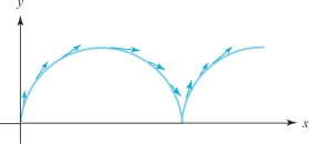
Figure 12.15 shows some velocity vectors superimposed on the cycloidal path of Figure 12.6.
Tangent Line
The tangent line to a path at a point is the line through the point in the direction of the tangent vector. Using the point-direction form of the equation of a line, we obtain the parametric equation for the tangent line.
Tangent Line to a Path
If \({\bf c}(t)\) is a path, and if \({\bf c'}(t_0)\ne 0\), the equation of its tangent line at the point \({\bf c}(t_0)\) is \[ \boldsymbol{\mathit{l}}(t)={\bf c}(t_0)+(t-t_0){\bf c}'(t_0). \]
If \(C\) is the curve traced out by \({\bf c}\), then the line traced out by l is the tangent line to the curve \(C\) at \({\bf c}(t_0)\).
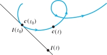
Notice that we have written the equation in such a way that l goes through the point \({\bf c}(t_0)\) at \(t=t_0\) (rather than \(t=0\)). See Figure 12.16.
example 8
A path in \({\mathbb R}^3\) goes through the point (3, 6, 5) at \(t=0\) with tangent vector \({\bf i}-{\bf j}\). Find the equation of the tangent line.
solution The equation of the tangent line is \[ \boldsymbol{\mathit{l}}(t)=(3,6,5)+t({\bf i}-{\bf j})=(3,6,5)+t(1,-1,0)=(3+t,6-t,5). \]
In \((x,y,z)\) coordinates, the tangent line is \(x=3+t,y=6-t,z=5\).
Physically, we can interpret motion along the tangent line as the path that a particle on a curve would follow if it were set free at a certain moment.
123
example 9
Suppose that a particle follows the path \({\bf c}(t)=(e^t,e^{-t},\cos t)\) until it flies off on a tangent at \(t=1\). Where is it at \(t=3\)?
solution The velocity vector is \((e^t, -e^{-t},{-}{\sin t})\), which at \(t=1\) is the vector \((e,-1/e,{-}{\sin 1})\). The particle is at \((e,1/e,\cos 1)\) at \(t=1\). The equation of the tangent line is \(\boldsymbol{\mathit{l}}(t)=(e,1/e,\cos 1)+(t-1)(e,-1/e,{-}{\sin 1})\). At \(t=3\), the position on this line is \begin{eqnarray*} \boldsymbol{\mathit{l}}(3) &=& \bigg(e,\frac{1}{e},\cos 1\bigg)+2\,\bigg(e,-\frac{1}{e},{-}{\sin 1}\bigg)=\bigg(3e,-\frac{1}{e},\cos 1-2\sin 1\bigg)\\[6pt] &\cong& (8.155,-0.368,-1.143). \\[-36pt] \end{eqnarray*}
Question 12.3 Section 12.1 Progress Check Question 3
Find an equation of the tangent line \({\bf l}(t)\) to the path \({\bf c}(t) = (1, t^2, t^3)\) at \(t=1\).
| A. |
| B. |
| C. |
| D. |
| E. |