13.3 Differentiation
In Section 13.1 we considered a few methods for graphing functions. By these methods alone it may be impossible to compute enough information to grasp even the general features of a complicated function. From elementary calculus, we know that the idea of the derivative can greatly aid us in this task; for example, it enables us to locate maxima and minima and to compute rates of change. The derivative also has many applications beyond this, as you have surely has discovered in elementary calculus.
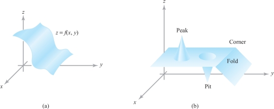
Intuitively, we know from our work in Section 13.2 that a continuous function is one that has no “breaks” in its graph. A differentiable function from \({\mathbb R}^2\) to \({\mathbb R}\) ought to be such that not only are there no breaks in its graph, but there is a well-defined plane tangent to the graph at each point. Thus, there must not be any sharp folds, corners, or peaks in the graph (see Figure 13.35). In other words, the graph must be smooth.
In Chapter 2 we defined the notion of a differentiable path \({\bf c}(t)\), which is a function of a single variable \(t\) but takes values in \(\mathbb{R}^n\), Euclidean \(n\)-space. The derivative \({\bf c}'(t)\) of such a path at time \(t\) is then a vector in \(\mathbb{R}^n\).
But what about functions \(f\), say, from \(\mathbb{R}^n\) to \(\mathbb{R}^m\)? What does it mean for \(f\) to be differentiable, and more importantly, what is the derivative of a differentiable function from \(\mathbb{R}^n\) to \(\mathbb{R}^m\)? It turns out that answers to these questions was necessary both for the development of mathematics as well as theoretical physics. Without such answers the development of the mathematical fields of differential topology, differential geometry, advanced mechanics and Einstein's General Theory of Relativity (about which we will later speak) would not have been possible.
The answers to what it means to be differentiable what a derivative actually is requires some insights. We begin with the more basic idea of a partial derivative of a real valued function of \(n\) variables.
Partial Derivatives
To make these ideas precise, we need a sound definition of what we mean by the phrase \({\rm “}f(x_1,\ldots, x_n)\) is differentiable at \({\bf x} = (x_1,\ldots ,x_n)\).” Actually, this definition is not quite as simple as one might think. Toward this end, however, let us introduce the notion of the partial derivative. This notion relies only on our knowledge of one-variable calculus. (A quick review of the definition of the derivative in a one-variable calculus text might be advisable at this point.)
106
Definition: Partial Derivatives
Let \(U\subset {\mathbb R}^n\) be an open set and suppose \(f\colon\, U\subset {\mathbb R}^n\rightarrow {\mathbb R}\) is a real-valued function. Then \(\partial f/\partial x_1,\ldots, \partial f/\partial x_n\), the partial derivatives of \(f\) with respect to the first, second, \(\ldots\) , \(n\)th variable, are the real-valued functions of \(n\) variables, which, at the point \((x_1,\ldots ,x_n)={\bf x}\), are defined by \begin{eqnarray*} \frac{\partial f}{\partial x_j} (x_1,\ldots ,x_n) &=& \lim_{h\rightarrow 0} \frac{f(x_1,x_2,\ldots,x_j+h,\ldots ,x_n)-f(x_1,\ldots ,x_n)}{h}\\ &=& \lim_{h\rightarrow 0}\frac{f({\bf x} + h {\bf e}_j)-f({\bf x})}{h} \end{eqnarray*} if the limits exist, where \(1\leq j\leq n\) and \({\bf e}_j\) is the \(j\)th standard basis vector defined by \({\bf e}_j=(0,\ldots, 1,\ldots, 0)\), with 1 in the \(j\)th slot (see Section 1.5). The domain of the function \(\partial f/\partial x_j\) is the set of \({\bf x}\in {\mathbb R}^n\) for which the limit exists.
In other words, \(\partial f/\partial x_j\) is just the derivative of \(f\) with respect to the variable \(x_j\), with the other variables held fixed. If \(f\colon\, {\mathbb R}^3\rightarrow {\mathbb R}\), we shall often use the notation \(\partial f/\partial x, \partial f/\partial y, \partial f/\partial z\) in place of \(\partial f/\partial x_1, \partial f/\partial x_2, \partial f/\partial x_3\). If \(f\colon\, U\subset {\mathbb R}^n\rightarrow {\mathbb R}^m\), then we can write \[ f(x_1,\ldots,x_n)=(f_1(x_1,\ldots,x_n),\ldots,f_m(x_1,\ldots,x_n)), \] so that we can speak of the partial derivatives of each component; for example, \(\partial f_m/\partial x_n\) is the partial derivative of the \(m\)th component with respect to \(x_n\), the \(n\)th variable.
example 1
If \(f(x,y)=x^2y+y^3,\) find \(\partial f/\partial x\) and \(\partial f/\partial y\).
solution To find \(\partial f/\partial x\) we hold \(y\) constant (think of it as some number, say 1) and differentiate only with respect to \(x\); this yields \[ \frac{\partial f}{\partial x}=\frac{\partial(x^2y+y^3)}{\partial{x}}=2xy. \]
Similarly, to find \(\partial f/\partial y\) we hold \(x\) constant and differentiate only with respect to \(y\): \[ \frac{\partial f}{\partial y}=\frac{\partial(x^2y+y^3)}{\partial y}=x^2+3y^2. \]
To indicate that a partial derivative is to be evaluated at a particular point, for example, at \((x_0,y_0)\), we write \[ \frac{\partial f}{\partial x}(x_0,y_0)\qquad\hbox{or} \qquad \frac{\partial f}{\partial x}\bigg|_{x=x_0,y=y_0} \qquad \hbox{or}\qquad \frac{\partial f}{\partial x}\bigg|_{(x_0,y_0)}. \]
When we write \(z=f(x,y)\) for the dependent variable, we sometimes write \(\partial z/\partial x\) for \(\partial f/\partial x\). Strictly speaking, this is an abuse of notation, but it is common practice to use these two notations interchangeably.
107
example 2
If \(z=\cos xy +x\cos y=f(x,y),\) find the two partial derivatives \((\partial z/\partial x)\) \((x_0,y_0)\) and \((\partial z/\partial y)(x_0,y_0)\).
solution First we fix \(y_0\) and differentiate with respect to \(x\), giving \begin{eqnarray*} \frac{\partial z}{\partial x} (x_0,y_0) &=& \frac{\partial(\cos xy_0+x\cos y_0)}{\partial x} \bigg|_{x=x_0}\\[2pt] &=&(-y_0\sin xy_0+\cos y_0)|_{x=x_0}\\[1pt] &=& - y_0\sin x_0y_0+\cos y_0. \end{eqnarray*}
Similarly, we fix \(x_0\) and differentiate with respect to \(y\) to obtain \begin{eqnarray*} \frac{\partial z}{\partial y} (x_0,y_0) &=& \frac{\partial(\cos x_0y+x_0\cos y)}{\partial y} \bigg|_{y=y_0}\\[2pt] &=&(-x_0\sin x_0y-x_0\sin y)|_{y=y_0}\\[1pt] &=&-x_0\sin x_0y_0-x_0\sin y_0. \\[-36pt] \end{eqnarray*}
example 3
Find \(\partial f/\partial x\) if \(f(x,y)=xy/\sqrt{x^2+y^2}\).
solution By the quotient rule, \[ \frac{\partial f}{\partial x} = \frac{y\sqrt{x^2+y^2}-xy(x/\sqrt{x^2+y^2})}{x^2+y^2}=\frac{y(x^2+y^2)-x^2y}{(x^2+y^2)^{3/2}} =\frac{y^3}{(x^2+y^2)^{3/2}}. \]
Question 13.83 Section 13.3 Progress Check Question 1
Let \(f(x,y)= \sin (xy) + x^2y\). Find the partial derivative \(\frac{\partial f}{\partial x}\).
| A. |
| B. |
| C. |
| D. |
| E. |
Sometimes the notation \(f_x, f_y, f_z\) is used for the partial derivatives: \(f_x=\dfrac{\partial f}{\partial x}, f_y= \dfrac{\partial f}{\partial y}, f_z=\dfrac{\partial f}{\partial z}\) and so on.
EXAMPLE 4
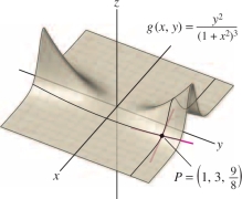
Calculate \(g_x(1,3)\) and \(g_y(1,3)\), where \(g(x,y)=\frac{y^2}{(1+x^2)^3}\).
Solution To calculate \(g_x\), treat \(y\) (and therefore \(y^2\)) as a constant: \[ \begin{array}{rl} g_x(x,y) &= \frac{\partial}{\partial x} \frac{y^2}{(1+x^2)^3} = y^2\frac{\partial}{\partial x} (1+x^2)^{-3}= \frac{-6xy^2}{(1+x^2)^4}\\ g_x(1,3)&= \frac{-6(1)3^2}{(1 + 1^2)^4} = -\frac{27}{8} \end{array} \] To calculate \(g_y\), treat \(x\) (and therefore \(1+x^2\)) as a constant: \begin{equation*} g_y(x,y) = \frac{\partial }{\partial y}\frac{y^2}{(1+x^2)^3} = \frac{1}{(1+x^2)^3}\frac{\partial }{\partial y}y^2 = \frac{2y}{(1+x^2)^3}\tag{1} \end{equation*} \[ g_y(1,3) = \frac{2(3)}{(1 + 1^2)^3} = \frac34 \]
CAUTION
It is not necessary to use the Quotient Rule to compute the partial derivative in Eq. (1). The denominator does not depend on \(y\), so we treat it as a constant when differentiating with respect to \(y\).
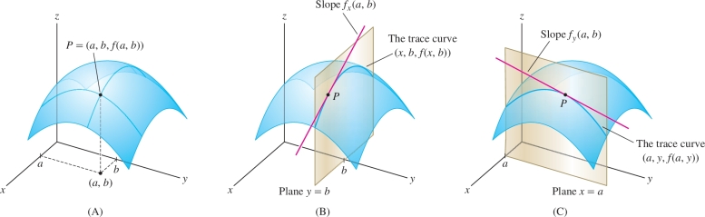
These partial derivatives are the slopes of the trace curves through the point \(\big(1,3,\frac98\big)\) shown in Figure 13.36.
796
EXAMPLE 5
Calculate \(f_z(0,0,1,1)\), where \[ f(x,y,z,w) = \frac{e^{xz+y}}{z^2+w} \]
Solution Use the Quotient Rule, treating \(x\), \(y\), and \(w\) as constants: \[ \begin{array}{rl} f_z(x,y,z,w) &= \frac{\partial}{\partial z}\left( \frac{e^{xz+y}}{z^2+w}\right) = \frac{(z^2+w)\frac{\partial}{\partial z} e^{xz+y}- e^{xz+y} \frac{\partial}{\partial z}(z^2+w)}{(z^2+w)^2} \\[6pt] &= \frac{(z^2+w)x e^{xz+y}- 2ze^{xz+y}}{(z^2+w)^2} = \frac{(z^2x+wx-2z)e^{xz+y}}{(z^2+w)^2}\\[6pt] f_z(0,0,1,1)&=\frac{-2e^0}{(1^2+1)^2}=-\frac12 \end{array} \]
In Example 5, the calculation \[ \frac{\partial}{\partial z} e^{xz+y}=xe^{xz+y} \] follows from the Chain Rule, just like \[ \frac{d }{d z} e^{az+b}=ae^{az+b} \]
Because the partial derivative \(f_x(a,b)\) is the derivative \(f(x,b)\), viewed as a function of \(x\) alone, we can estimate the change \(\Delta f\) when \(x\) changes from \(a\) to \(a+\Delta x\) as in the single-variable case. Similarly, we can estimate the change when \(y\) changes by \(\Delta y\). For small \(\Delta x\) and \(\Delta y\) (just how small depends on \(f\) and the accuracy required): \[ \boxed{\begin{array}{rcl} f(a+\Delta x,b) -f(a,b)\,\,&\approx&\,\, f_x(a,b)\Delta x \\ \\ f(a,b+\Delta y) -f(a,b)\,\,&\approx&\,\, f_y(a,b)\Delta y \end{array}} \]
This applies to functions \(f\) in any number of variables. For example, \(\Delta f \approx f_w \Delta w\) if one of the variables \(w\) changes by \(\Delta w\) and all other variables remain fixed.
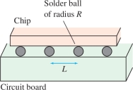
EXAMPLE 6 Testing Microchips
A ball grid array (BGA) is a microchip joined to a circuit board by small solder balls of radius \(R\) mm separated by a distance \(L\) mm (Figure 13.37). Manufacturers test the reliability of BGAs by subjecting them to repeated cycles in which the temperature is varied from \(0^\circ\)C to \(100^\circ\)C over a 40-min period. According to one model, the average number \(N\) of cycles before the chip fails is \[ N = \left(\frac{2200R}{Ld} \right)^{1.9} \] where \(d\) is the difference between the coefficients of expansion of the chip and the board. Estimate the change \(\Delta N\) when \(R=0.12\), \(d = 10\), and \(L\) is increased from 0.4 to 0.42.
Solution We use the approximation \[ \Delta N \approx \frac{\partial N}{\partial L}\,\Delta L \] with \(\Delta L = 0.42-0.4 = 0.02\). Since \(R\) and \(d\) are constant, the partial derivative is \[ \frac{\partial N}{\partial L} = \frac{\partial}{\partial L} \left(\frac{2200R}{Ld} \right)^{1.9} = \left(\frac{2200R}{d} \right)^{1.9}\frac{\partial}{\partial L} L^{-1.9} = -1.9\left(\frac{2200R}{d} \right)^{1.9}L^{-2.9} \]
797
Now evaluate at \(L=0.4\), \(R=0.12\), and \(d=10\): \[ \frac{\partial N}{\partial L}\bigg|_{(L,R,d)=(0.4,0.12,10)} = -1.9\left(\frac{2200(0.12)}{10} \right)^{1.9}(0.4)^{-2.9}\approx -13{,}609 \]
The decrease in the average number of cycles before a chip fails is \[ \Delta N \approx \frac{\partial N}{\partial L}\Delta L =-13{,}609(0.02)\approx -272~\mathrm{cycles} \]
We can interpret the meaning of the partial derivatives \(f_x(a,b), f_y(a,b)\) geometrically in terms of the curves (or traces) which result from the intersection of the graph of \(f\) with the vertical planes through the point \((a,b,f(a,b))\) parallel to the \((x,z)\) and \((y,z)\) planes respectively, as depicted in the figure below.
It is important to understand that a definition of differentiability that requires only the existence of partial derivatives turns out to be insufficient. Many standard results, such as the chain rule for functions of several variables, would not follow, as Example 4 shows. Below, we shall see how to rectify this situation.
example 7
Let \(f(x,y)=x^{1/3}y^{1/3}\). By definition, \[ \frac{\partial f}{\partial x}(0,0)=\mathop {{\rm limit}\ }_{h\rightarrow 0} \frac{f(h,0)-f(0,0)}{h}=\mathop {{\rm limit}\ }_{h\rightarrow 0} \frac{0-0}{h}=0, \] and, similarly, \((\partial f/\partial y)(0,0)=0\) (these are not indeterminate forms!). It is necessary to use the original definition of partial derivatives, because the functions \(x^{1/3}\) and \(y^{1/3}\) are not themselves differentiable at 0. Suppose we restrict \(f\) to the line \(y\,{=}\,x\) to get \(f(x,x)=x^{2/3}\) (see Figure 13.39). We can view the substitution \(y=x\) as the composition \(f\circ g\) of the function \(g\colon\, {\mathbb R} \rightarrow {\mathbb R}^2\), defined by \(g(x)=(x,x)\), and \(f\colon\, {\mathbb R}^2\rightarrow {\mathbb R},\) defined by \(f(x,y)=x^{1/3}y^{1/3}\).
Thus, the composite \(f\circ g\) is given by \((f\circ g)(x)=x^{2/3}\). Each component of \(g\) is differentiable in \(x\), and \(f\) has partial derivatives at \((0,0),\) but \(f\circ g\) is not differentiable at \(x=0\), in the sense of one-variable calculus. In other words, the composition of \(f\) with \(g\) is not differentiable in contrast to the calculus of functions of one variable, where the composition of differentiable functions is differentiable. Later, we shall give a definition of differentiability that has the pleasant consequence that the composition of differentiable functions is differentiable.
There is another reason for being dissatisfied with the mere existence of partial derivatives of \(f(x,y)=x^{1/3}y^{1/3}\): There is no plane tangent, in any reasonable sense, to the graph at \((0, 0)\). The \(xy\) plane is tangent to the graph along the \(x\) and \(y\) axes because \(f\) has slope zero at \((0, 0)\) along these axes; that is, \(\partial f/\partial x=0\) and \(\partial f/\partial y=0\) at \((0, 0)\).
108
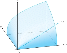
Thus, if there is a tangent plane, it must be the \(xy\) plane. However, as is evident from Figure 13.39, the \(xy\) plane is not tangent to the graph in other directions, because the graph has a severe crinkle, and so the \(xy\) plane cannot be said to be tangent to the graph of \(f\).
The Linear or Affine Approximation
To “motivate” our definition of differentiability, let us compute what the equation of the plane tangent to the graph of \(f\colon \,{\mathbb R}^2\rightarrow {\mathbb R}, (x,y)\mapsto f(x,y)\) at \((x_0,y_0)\) ought to be if \(f\) is smooth enough. In \({\mathbb R}^3\), a nonvertical plane has an equation of the form \[ z=ax+by+c. \]
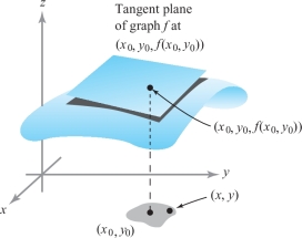
If it is to be the plane tangent to the graph of \(f\), the slopes along the \(x\) and \(y\) axes must be equal to \(\partial f/\partial x\) and \(\partial f/\partial y\), the rates of change of \(f\) with respect to \(x\) and \(y\). Thus, \(a=\partial f/\partial x, b=\partial f/\partial y\) [evaluated at \((x_0,y_0)\)]. Finally, we may determine the constant \(c\) from the fact that \(z=f(x_0,y_0)\) when \(x=x_0,y=y_0\). Thus, we get the linear approximation (or, more accurately said, affine approximation): \begin{equation} z=f(x_0,y_0)+\bigg[\frac{\partial f}{\partial x}(x_0,y_0)\bigg](x-x_0)+ \bigg[\frac{\partial f}{\partial y}(x_0,y_0)\bigg](y-y_0), \end{equation} which should be the equation of the plane tangent to the graph of \(f\) at \((x_0,y_0)\), if \(f\) is “smooth enough” (see Figure 13.40).
Our definition of differentiability will mean in effect that the plane defined by the linear approximation (1) is a “good” approximation of \(f\) near \((x_0,y_0)\). To get an idea of what we might mean by a good approximation, let us return for a moment to one-variable calculus. If \(f\) is differentiable at a point \(x_0\), then we know that \[ \mathop {{\rm limit}\ }_{\Delta x \rightarrow 0} \frac{f(x_0+\Delta x)-f(x_0)}{\Delta x}=f'(x_0). \]
Let \(x=x_0+\Delta x\) and rewrite this as \[ \mathop {{\rm limit}\ }_{x \rightarrow x_0} \frac{f(x)-f(x_0)}{x-x_0}=f'(x_0). \]
Using the trivial limit \({\rm limit}_{x\rightarrow x_0}f'(x_0)=f'(x_0)\), we can rewrite the preceding equation as \[ \mathop {{\rm limit}\ }_{x \rightarrow x_0} \frac{f(x)-f(x_0)}{x-x_0}= \mathop {{\rm limit}\ }_{x\rightarrow x_0}f'(x_0); \] that is, \[ \mathop {{\rm limit}\ }_{x \rightarrow x_0} \bigg[\frac{f(x)-f(x_0)}{x-x_0}-f'(x_0)\bigg]=0; \] that is, \[ \mathop {{\rm limit}\ }_{x \rightarrow x_0} \frac{f(x)-f(x_0)-f'(x_0)(x-x_0)}{x-x_0}=0. \]
109
Thus, the tangent line \(l\) through \((x_0,f(x_0))\) with slope \(f'(x_0)\) is close to \(f\) in the sense that the difference between \(f(x)\) and \(l(x)=f(x_0)+f'(x_0)(x-x_0)\), the equation of the tangent line goes to zero even when divided by \(x -{x_0}\) as \(x\) goes to \(x_0\). This is the notion of a “good approximation” that we will adapt to functions of several variables, with the tangent line replaced by the tangent plane [see equation (1), given earlier].
Differentiability for Functions of Two Variables
Using the linear approximation, we are ready to define the notion of differentiability.
Definition: Differentiable: Two Variables
Let \(f\colon\, {\mathbb R}^2\rightarrow\) \({\mathbb R}\). We say \(f\) is differentiable at \((x_0,y_0)\), if \(\partial f/\partial x\) and \(\partial f/\partial y\) exist at \((x_0,y_0)\) and if \begin{equation} \frac{f(x,y)-f(x_0,y_0)- \displaystyle\bigg[\frac{\partial f}{\partial x}(x_0,y_0)\bigg](x-x_0)- \displaystyle\bigg[\frac{\partial f}{\partial y}(x_0,y_0)\bigg](y-y_0)} { \| (x,y)-(x_0,y_0) \| }\,\rightarrow 0 \end{equation} as \((x,y)\rightarrow (x_0,y_0)\). This equation expresses what we mean by saying that \[ f(x_0,y_0)+\bigg[\frac{\partial f}{\partial x}(x_0,y_0)\bigg](x-x_0)+ \bigg[\frac{\partial f}{\partial y}(x_0,y_0)\bigg](y-y_0) \] is a good approximation to the function \(f\), also called a linear approximation.
It is not always easy to use this definition to see whether \(f\) is differentiable, but it will be easy to use another criterion, given shortly in Theorem 9.
Tangent Plane
110
We have used the informal notion of the plane tangent to the graph of a function to motivate our definition of differentiability. Now we are ready to adopt a formal definition of the tangent plane.
Definition: Tangent Plane
Let \(f\colon\, {\mathbb R}^{\smash{2}}\rightarrow\, {\mathbb R}\) be differentiable at \({\bf x}_0=(x_0,y_0)\). The plane in \({\mathbb R}^3\) defined by the equation \[ z=f(x_0,y_0)+\bigg[\frac{\partial f}{\partial x}(x_0,y_0)\bigg](x-x_0)+ \bigg[\frac{\partial f}{\partial y}(x_0,y_0)\bigg](y-y_0) \] is called the tangent plane of the graph of \(f\) at the point \((x_0,y_0, f(x_0,y_0))\).
example 8
Compute the plane tangent to the graph of \(z=x^2+y^4+e^{xy}\) at the point \((1, 0, 2).\)
solution Use formula (1), with \(x_0=1,y_0=0\), and \(z_0=f(x_0,y_0)\,{=}\,2\). The partial derivatives are \[ \frac{\partial z}{\partial x}=2x+ye^{xy} \qquad \hbox{and} \qquad \frac{\partial z}{\partial y}=4y^3+xe^{xy}. \]
At (1, 0, 2), these partial derivatives are 2 and 1, respectively. Thus, by formula (1), the tangent plane is \[ z=2(x-1) +1(y-0)+2,\hbox{that is,}\qquad z=2x+y. \]
Let us write \({\bf D} f(x_0,y_0)\) for the row matrix \[ \bigg[\frac{\partial f}{\partial x}(x_0,y_0)\quad \frac{\partial f}{\partial y} (x_0,y_0) \bigg], \] so that the definition of differentiability asserts that \begin{equation} \begin{array}{l} f(x_0,y_0)+{\bf D} f(x_0,y_0) \Big[ \begin{array}{c} x-x_0\\ y-y_0 \end{array} \Big]\\ \quad =f(x_0,y_0)+\bigg[ \frac{\partial f}{\partial x}(x_0,y_0) \bigg](x-x_0) + \bigg[\frac{\partial f}{\partial y} (x_0,y_0) \bigg](y-y_0) \end{array} \end{equation} is our good approximation to \(f\) near \((x_0,y_0)\). As earlier, “good” is taken in the sense that expression (3) differs from \(f(x,y)\) by something small times \(\sqrt{(x-x_0)^2 + (y-y_0)^2}\). We say that expression (3) is the best linear approximation to \(f\) near \((x_0,y_0)\).
Best linear approximation means that near \((x_0, y_0, f(x_0,y_0))\), the surface is closely approximated by the tangent plane; we sometimes say that \(f(x,y)\) is locally linear near \((x_0, y_0, f(x_0,y_0))\).
The next example shows again that the existence of the partial derivatives is not sufficient to guarantee the existence of a tangent plane as a linear approximation.
example 9
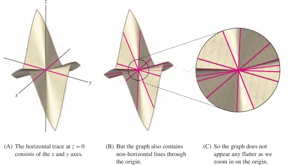
Consider \(g(x,y)=\dfrac{2xy(x+y)}{x^2+y^2}\). The graph contains the \(x\)- and \(y\)-axes—in other words, \(g(x,y) =0\) if \(x\) or \(y\) is zero—and therefore, the partial derivatives \(g_x(0,0)\) and \(g_y(0,0)\) are both zero. The tangent plane at the origin \((0,0)\), if it existed, would have to be the \(xy\)-plane. However, Figure 13.41(B) below shows that the graph also contains lines through the origin that do not lie in the \(xy\)-plane (in fact, the graph is composed entirely of lines through the origin). As we zoom in on the origin, these lines remain at an angle to the \(xy\)-plane, and the surface does not get any flatter. Thus \(g(x,y)\) cannot be locally linear at \((0,0)\), and the tangent plane does not exist, i.e. \(g\) is not differentiable at the origin.
The Derivative and Differentiability: The General Case
Now we are ready to give a definition of differentiability for maps \(f\) of \({\mathbb R}^n\) to \({\mathbb R}^m\), using the preceding discussion as motivation. The derivative \({\bf D} f({\bf x}_0)\) of \(f=(f_1,\ldots ,f_m)\) at a point \({\bf x}_0\) is a matrix \({\bf T}\) whose elements are \(t_{ij}=\partial f_i/\partial x_j\) evaluated at \({\bf x}_0\).footnote #
111
Definition: Differentiable, \(n\) Variables, \(m\) Functions
Let \(U\) be an open set in \({\mathbb R}^n\) and let \(f\colon\, U\subset {\mathbb R}^n\rightarrow {\mathbb R}^m\) be a given function. We say that \(f\) is differentiable at \({\bf x}_0\in U\) if the partial derivatives of \(f\) exist at \({\bf x}_0\) and if \begin{equation} \mathop {{\rm limit}\ }_{{\bf x}\rightarrow {\bf x}_0} \frac{ \| f({\bf x})-f({\bf x}_0)-{\bf T}({\bf x}- {\bf x}_0) \| }{ \| {\bf x}-{\bf x}_0 \| }= 0, \end{equation} where \({\bf T}={\bf D} f({\bf x}_0)\) is the \(m\times n\) matrix with matrix elements \(\partial f_i/\partial x_j\) evaluated at \({\bf x}_0\) and \({\bf T}({\bf x}-{\bf x}_0)\) means the product of T with \({\bf x}- {\bf x}_0\) (regarded as a column matrix). We call T the derivative of \(f\) at \({\bf x}_0\).
We shall always denote the derivative \({\bf T}\) of \(f\) at \({\bf x}_0\) by \({\bf D}f({\bf x}_0)\), although in some books it is denoted \(df({\bf x}_0)\) and referred to as the differential of \(f\). In the case where \(m=1\), the matrix \({\bf T}\) is just the row matrix \[ \bigg[ \frac{\partial f}{\partial x_1}({\bf x}_0)\quad\cdots \quad \frac{\partial f}{\partial x_n}({\bf x}_0) \bigg] . \] (Sometimes, when there is danger of confusion, we separate the entries by commas.) Furthermore, setting \(n=2\) and putting the result back into equation (4), we see that conditions (2) and (4) do agree. Thus, if we let \({\bf h}={\bf x}-{\bf x}_0\), a real-valued function \(f\) of \(n\) variables is differentiable at a point \({\bf x}_0\) if \[ \mathop {{\rm limit}\ }_{{\bf h}\rightarrow 0}\frac{1}{ \| {\bf h} \| } \bigg|f({\bf x}_0+{\bf h})-f({\bf x}_0) -\sum^n_{j=1} \frac{\partial f}{\partial x_j}({\bf x}_0)h_j\bigg|=0, \] because \[ {\bf Th}=\sum^n_{j=1}h_j \frac{\partial f}{\partial x_j}({\bf x}_0). \]
For the general case of \(f\) mapping a subset of \({\mathbb R}^n\) to \({\mathbb R}^m\), the derivative is the \(m\times n\) matrix given by \[ {\bf D} f({\bf x}_0)=\left[ \begin{array}{c@{\quad}c@{\quad}c} \displaystyle \frac{\partial f_1}{\partial x_1} & \cdots & \displaystyle \frac{\partial f_1}{\partial x_n}\\ \vdots & &\vdots \\[3pt] \displaystyle \frac{\partial f_m}{\partial x_1} & \cdots & \displaystyle \frac{\partial f_m}{\partial x_n} \end{array}\right], \] where \(\partial f_i/\partial x_j\) is evaluated at \({\bf x}_0\). The matrix \({\bf D} f({\bf x}_0)\) is, appropriately, called the matrix of partial derivatives of \(f\) at \({\bf x}_0\).
example 10
Calculate the matrices of partial derivatives for these functions.
- (a) \(f(x,y)=(e^{x+y}+y,y^2x)\)
- (b) \(f(x,y)=(x^2+\cos y, ye^x)\)
- (c) \(f(x,y,z)=\) \((ze^x,-ye^z)\)
112
solution
- (a) Here \(f\colon\, {\mathbb R}^2 \rightarrow {\mathbb R}^2\) is defined by \(f_1(x,y)=e^{x+y}+y\) and \(f_2(x,y)=y^2x\). Hence, \({\bf D} f(x,y)\) is the \(2\times 2\) matrix \[ {\bf D} f(x,y)=\bigg[ \begin{array}{c@{\quad}c} e^{x+y}&e^{x+y} + 1\\ y^2&2xy \end{array} \bigg]. \]
- (b) We have \[ {\bf D} f(x,y)=\bigg[ \begin{array}{c@{\quad}c} 2x & {-}{\sin y}\\ ye^x& e^x \end{array} \bigg]. \]
- (c) In this case, \[ {\bf D} f(x,y,z)=\bigg[ \begin{array}{c@{\quad}c@{\quad}c} ze^x & 0 &e^x\\ 0 &-e^z &-ye^z \end{array} \bigg]. \]
Gradients
For real-valued functions we use special terminology for the derivative.
Definition: Gradient
Consider the special case \(f\colon\, U\subset {\mathbb R}^n\rightarrow {\mathbb R}\). Here \({\bf D} f({\bf x})\) is a \(1\times n\) matrix: \[ {\bf D} f({\bf x})=\bigg[ \frac{\partial f}{\partial x_1}\quad \cdots\quad \frac{\partial f}{\partial x_n} \bigg]. \]
We can form the corresponding vector \((\partial f/\partial x_1,\ldots ,\partial f/\partial x_n),\) called the gradient of \(f\) and denoted by \({\nabla } f\), or grad \(f\).
From the definition, we see that for \(f\colon\, {\mathbb R}^3\rightarrow {\mathbb R}\), \[ {\nabla} f=\frac{\partial f}{\partial x}{\bf i}+\frac{\partial f}{\partial y}{\bf j}+ \frac{\partial f}{\partial z}{\bf k}, \] while for \(f\colon\, {\mathbb R}^2\rightarrow {\mathbb R}\), \[ {\nabla} f=\frac{\partial f}{\partial x}{\bf i}+\frac{\partial f}{\partial y}{\bf j}. \]
The geometric significance of the gradient will be discussed in Section 13.5. In terms of inner products, we can write the derivative of \(f\) as \[ {\bf D} f({\bf x})({\bf h})={\nabla} f({\bf x})\,{ \cdot}\, {\bf h}. \]
example 11
Let \(f\colon\, {\mathbb R}^3\rightarrow {\mathbb R},f(x,y,z)=xe^y\). Then \[ {\nabla} f=\bigg(\frac{\partial f}{\partial x},\frac{\partial f}{\partial y}, \frac{\partial f}{\partial z} \bigg)=(e^y,xe^y,0). \]
113
example 12
If \(f\colon \,{\mathbb R}^2\rightarrow {\mathbb R}\) is given by \((x,y)\mapsto e^{xy}+\sin xy,\) then \begin{eqnarray*} {\nabla} f(x,y) &=& (ye^{xy}+y\cos xy){\bf i}+(xe^{xy}+x\cos xy){\bf j}\\ &=&(e^{xy}+\cos xy)(y{\bf i}+x{\bf j}).\\[-36pt] \end{eqnarray*}
In one-variable calculus it is shown that if \(f\) is differentiable, then \(f\) is continuous. We will state in Theorem 8 that this is also true for differentiable functions of several variables. As we know, there are plenty of functions of one variable that are continuous but not differentiable, such as \(f(x)=|x|\). Before stating the result, let us give an example of a function of two variables whose partial derivatives exist at a point, but which is not continuous at that point.
example 13
Let \(f\colon\, {\mathbb R}^2\rightarrow {\mathbb R}\) be defined by \[ f(x,y)=\bigg\{ \begin{array}{c@{\qquad}l} 1&\hbox{if } x= 0 \hbox{ or if } y = 0\\[1pt] 0&\hbox{otherwise}. \end{array} \]
Because \(f\) is constant on the \(x\) and \(y\) axes, where it equals 1, \[ \frac{\partial f}{\partial x}(0,0)=0\qquad \hbox{and} \qquad \frac{\partial f}{\partial y}(0,0)=0. \]
But \(f\) is not continuous at \((0, 0),\) because \({\rm limit}_{(x,y) \,\to\, (0,0)} f(x,y)\) does not exist.
Some Basic Theorems
The first of these basic theorems relates differentiability and continuity.
Theorem 8
Let \(f\colon\, U\subset {\mathbb R}^n\rightarrow {\mathbb R}^m\) be differentiable at \({\bf x}_0\in U\). Then \(f\) is continuous at \({\bf x}_0\).
This result is very reasonable, because “differentiability" means that there is enough smoothness to have a tangent plane, which is stronger than just being continuous. Consult the Internet supplement for Chapter 2 for the formal proof.
As we have seen, it is usually easy to tell when the partial derivatives of a function exist using what we know from one-variable calculus. However, the definition of differentiability looks somewhat complicated, and the required approximation condition in equation (4) may seem, and sometimes is, difficult to verify. Fortunately, there is a simple criterion, given in the following theorem, that tells us when a function is differentiable.
Theorem 9
Let \(f\colon\, U\subset {\mathbb R}^n\rightarrow {\mathbb R}^m\). Suppose the partial derivatives \(\partial f_i/\partial x_j\) of \(f\) all exist and are continuous in a neighborhood of a point \({\bf x} \in U\). Then \(f\) is differentiable at \({\bf x}\).
114
We give the proof in the Internet supplement for Chapter 2. Notice the following hierarchy:
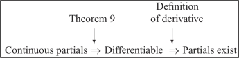
Each converse statement, obtained by reversing an implication, is invalid. [For a counterexample to the converse of the first implication, use \(f(x)=x^2\sin\, (1/x),\) \(f(0)=0\); for the second, see Example 1 in the Internet supplement for Chapter 2 or use Example 4 in this section.]
A function whose partial derivatives exist and are continuous is said to be of class \(C^1\). Thus, Theorem 9 says that any \(C^1\) function is differentiable.
example 14
Let \[ f(x,y)=\frac{\cos x+e^{xy}}{x^2+y^2}. \]
Show that \(f\) is differentiable at all points \((x,y)\not=(0,0)\).
solution Observe that the partial derivatives \begin{eqnarray*} \frac{\partial f}{\partial x}&=& \frac{(x^2+y^2)(ye^{xy}-\sin x)-2x(\cos x+e^{xy})} {(x^2+y^2)^2}\\[3pt] \frac{\partial f}{\partial y}&=& \frac{(x^2+y^2)xe^{xy}-2y(\cos x+e^{xy})} {(x^2+y^2)^2} \end{eqnarray*} are continuous except when \(x=0\) and \(y=0\) (by the results in Section 13.2). Thus, \(f\) is differentiable by Theorem 9.
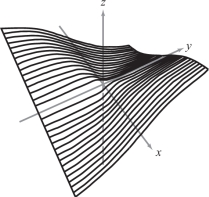
One can show that \(f(x,y)=xy/\sqrt{x^2+y^2}\) [with \(f(0,0)\,{=}\,0\)] is continuous, has partial derivatives at (0, 0), yet is not differentiable there. See Figure 13.42. By Theorem 9, its partial derivatives cannot be continuous at (0, 0).
EXAMPLE 15
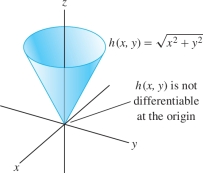
Where is \(h(x,y) =\sqrt{x^2+y^2}\) differentiable?
Solution The partial derivatives exist and are continuous for all \((x,y)\ne (0,0)\): \[ h_x(x,y) = \frac{x}{\sqrt{x^2+y^2}} ,\qquad h_y(x,y) = \frac{y}{\sqrt{x^2+y^2}} \]
However, the partial derivatives do not exist at \((0,0)\). Indeed, \(h_x(0,0)\) does not exist because \(h(x,0) = \sqrt{x^2}=|x|\) is not differentiable at \(x=0\). Similarly, \(h_y(0,0)\) does not exist. By Theorem 9, \(h(x,y)\) is differentiable except at \((0,0)\) (Figure 13.43).