3.5 The Implicit Function Theorem [Optional]
In this section we state two versions of the implicit function theorem, arguably the most important theorem in all of mathematical analysis. The entire theoretical basis of the idea of a surface as well as the method of Lagrange multipliers depends on it. Moreover, it is a cornerstone of several fields of mathematics, such as differential topology and geometry.
The One-Variable Implicit Function Theorem
In one-variable calculus we learn the importance of the inversion process. For example, \(x=\ln y\) is the inverse of \(y=e^x\), and \(x=\sin^{-1}y\) is the inverse of \(y=\sin x\). The inversion process is also important for functions of several variables; for example, the switch between Cartesian and polar coordinates in the plane involves inverting two functions of two variables.
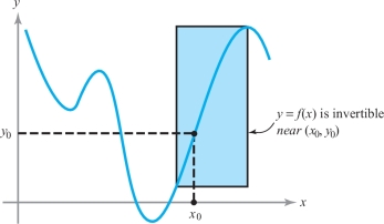
Recall from one-variable calculus that if \(y\,{=}\,f(x)\) is a \(C^1\) function and \(f'(x_0)\,{\neq}\,0\), then locally near \(x_0\) we can solve for \(x\) to give the inverse function: \(x=f^{-1}(y)\). We learn that \((f^{-1})'(y)=1/f'(x)\); that is, \(dx/dy=1/(dy/dx)\). That \(y=f(x)\) can be inverted is plausible because \(f'(x_0) \neq 0\) means that the slope of \(y=f(x)\) is nonzero, so that the graph is rising or falling near \(x_0\). Thus, if we reflect the graph across the line \(y=x\), it is still a graph near \((x_0,y_0)\), where \(y_0=f(x_0)\). For example, in Figure 3.21, we can invert \(y=f(x)\) in the shaded box, so in this range, \(x=f^{-1}(y)\) is defined.
A Special Result
We next turn to the situation for real-valued functions of variables \(x_1,\ldots,x_n\) and \(z\).
204
Theorem 11 Special Implicit Function Theorem
Suppose that \(F\colon\, {\mathbb R}^{n+1} \rightarrow {\mathbb R}\) has continuous partial derivatives. Denoting points in \({\mathbb R}^{n+1}\) by \(({\bf x}, z),\) where \({\bf x}\in {\mathbb R}^n\) and \(z\in {\mathbb R},\) assume that \(({\bf x}_0,z_0)\) satisfies \[ F({\bf x}_0, z_0) = 0 \quad\hbox{and}\quad \frac{\partial F}{\partial z}({\bf x}_0,z_0) \neq 0. \]
Then there is a ball \(U\) containing \({\bf x}_0\) in \({\mathbb R}^n\) and a neighborhood \(V\) of \(z_0\) in \({\mathbb R}\) such that there is a unique function \(z=g({\bf x})\) defined for \({\bf x}\) in \(U\) and \(z\) in \(V\) that satisfies \[ F({\bf x},g({\bf x}))=0. \]
Moreover, if \({\bf x}\) in \(U\) and \(z\) in \(V\) satisfy \(F({\bf x}, z)=0,\) then \(z=g({\bf x})\). Finally, \(z=g({\bf x})\) is continuously differentiable, with the derivative given by \[ {\bf D}g({\bf x}) = - \frac{1}{\displaystyle \frac{\partial F}{\partial z}({\bf x}, z)}\,{\bf D}_{\bf x}F ({\bf x},z)\Bigg| _{z=g({\bf x})}, \] where \({\bf D}_{\bf x}F\) denotes the \((\)partial\()\) derivative of \(F\) with respect to the variable \({\bf x}\)—that is, we have \({\bf D}_{\bf x}F=[\partial F/ \partial x_1,\ldots, \partial F/\partial x_n];\) in other words, \begin{equation*} \frac{\partial g}{\partial x_i}=- \frac{\partial F/\partial x_i} {\partial F/\partial z}, \qquad i=1,\ldots,n.\tag{1} \end{equation*}
A proof of this theorem is given in the Internet supplement.
Once it is known that \(z=g({\bf x})\) exists and is differentiable, formula (1) may be checked by implicit differentiation; to see this, note that the chain rule applied to \(F({\bf x}, g({\bf x})) = 0\) gives \[ {\bf D}_{\bf x}F({\bf x}, g({\bf x})) + \bigg[ \frac{\partial F}{\partial z}({\bf x},g({\bf x}))\bigg] [{\bf D}g({\bf x})] = 0, \] which is equivalent to formula (1).
205
example 1
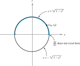
In the special implicit function theorem, it is important to recognize the necessity of taking sufficiently small neighborhoods \(U\) and \(V\). For example, consider the equation \[ x^2 + z^2 -1 =0; \] that is, \(F(x,z) = x^2 + z^2 -1\), with \(n=1\). Here \((\partial F/\partial z)(x,z)= 2z\), and so the special implicit function theorem applies to a point \((x_0,z_0)\), satisfying \(x^2_0 + z^2_0 -1 = 0\) and \(z_0 \neq 0\). Thus, near such points, \(z\) is a unique function of \(x\). This function is \(z= {\textstyle\sqrt{1-x^2}}\) if \(z_0 >0\) and \(z= -{\textstyle\sqrt{1-x^2}}\) if \(z_0< 0\). Note that \(z\) is defined for \({\mid} x{\mid} < 1\) only (\(U\) must not be too big) and \(z\) is unique only if it is near \(z_0\) \((V\) must not be too big\()\). These facts and the nonexistence of \(\partial z/\partial x\) at \(z_0=0\) are, of course, clear from the fact that \(x^2 + z^2 =1\) defines a circle in the \(xz\) plane (Figure 3.22).
The Implicit Function Theorem and Surfaces
Let us apply Theorem 11 to the study of surfaces. We are concerned with the level set of a function \(g{:}\,\, U \subset {\mathbb R}^{n}\rightarrow {\mathbb R}\); that is, with the surface \(S\) consisting of the set of \({\bf x}\) satisfying \(g({\bf x})=c_0 \), where \(c_0 = g({\bf x}_0)\) and where \({\bf x}_0\) is given. Let us take \(n=3\) for concreteness. Thus, we are dealing with the level surface of a function \(g(x,y,z)\) through a given point \((x_0,y_0,z_0)\). As in the Lagrange multiplier theorem, assume that \({\nabla}\! g(x_0,y_0,z_0)\neq {\bf 0}\). This means that at least one of the partial derivatives of \(g\) is nonzero. For definiteness, suppose that \((\partial g/\partial z)(x_0,y_0,z_0)\neq 0\). By applying Theorem 11 to the function \((x,y,z)\mapsto g(x,y,z)-c_0\), we know there is a unique function \(z=k(x,y)\) satisfying \(g(x,y,k(x,y))=c_0\) for \((x,y)\) near \((x_0,y_0)\) and \(z\) near \(z_0\). Thus, near \(z_0\) the surface \(S\) is the graph of the function \(k\). Because \(k\) is continuously differentiable, this surface has a tangent plane at \((x_0,y_0,z_0)\) given by \begin{equation*} z=z_0 + \bigg[ \frac{\partial k}{\partial x}(x_0,y_0)\bigg] (x - x_0) + \bigg[ \frac{\partial k}{\partial y} (x_0,y_0)\bigg] (y - y_0).\tag{2} \end{equation*}
But by formula (1), \[ \frac{\partial k}{\partial x}(x_0,y_0) = -\frac{\displaystyle \frac{\partial g}{\partial x}(x_0,y_0,z_0)}{\displaystyle \frac{\partial g}{\partial z}(x_0,y_0,z_0)}\quad \hbox{and}\quad \frac{\partial k}{\partial y}(x_0,y_0) = - \frac{\displaystyle \frac{\partial g}{\partial y}(x_0,y_0,z_0)}{\displaystyle \frac{\partial g}{\partial z}(x_0,y_0,z_0)}. \]
206
Substituting these two equations into the equation for the tangent plane gives this equivalent description: \[ 0= (z-z_0) \frac{\partial g}{\partial z}(x_0,y_0,z_0) + (x - x_0) \frac{\partial g}{\partial x}(x_0,y_0,z_0) + (y-y_0) \frac{\partial g}{\partial y}(x_0,y_0,z_0); \] that is, \[ (x-x_0,y-y_0,z-z_0) \,{\cdot} \, {\nabla} g(x_0,y_0,z_0) = 0. \]
Thus, the tangent plane to the level surface of \(g\) is the orthogonal complement to \({\nabla}\! g(x_0,y_0,z_0)\) through the point \((x_0,y_0,z_0)\). This agrees with our characterization of tangent planes to level sets from Chapter 2.
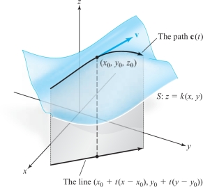
We are now ready to complete the proof of the Lagrange multiplier theorem. To do this, we must show that every vector tangent to \(S\) at \((x_0,y_0,z_0)\) is tangent to a curve in \(S\). By Theorem 11, we need only show this for a graph of the form \(z=k(x,y)\). However, if \({\bf v}= (x-x_0,y-y_0,z-z_0)\) is tangent to the graph [that is, if it satisfies equation (2)], then \({\bf v}\) is tangent to the path in \(S\) given by \[ {\bf c}(t) = (x_0 + t(x-x_0), y_0 + t(y-y_0), k(x_0+ t(x-x_0), y_0 + t(y-y_0))) \] at \(t=0\). This can be checked by using the chain rule. (See Figure 3.23.)
example 2
Near what points may the surface \[ x^3 +3y^2 + 8xz^2 - 3z^3 y =1 \] be represented as a graph of a differentiable function \(z=k(x,y)?\)
solution Here we take \(F(x,y,z)=x^3 +3y^2 +8xz^2 -3z^3y -1\) and attempt to solve \(F(x,y,z)=0\) for \(z\) as a function of \((x,y)\). By Theorem 11, this may be done near a point \((x_0,y_0,z_0)\) if \((\partial F/\partial z)(x_0,y_0,z_0)\neq 0\), that is, if \[ z_0(16x_0 - 9z_0 y_0) \neq 0, \] which means, in turn, \[ z_0 \neq 0 \qquad \hbox{and} \qquad 16x_0 \neq 9z_0 y_0. \]
General Implicit Function Theorem
207
Next we shall state, without proof, the general implicit function theorem.footnote # Instead of attempting to solve one equation for one variable, we attempt to solve \(m\) equations for \(m\) variables \(z_1,\ldots,z_m\): \begin{equation*} \begin{array}{r@{\,}c@{\,}l} F_1 (x_1,\ldots, x_n,z_1,\ldots,z_m) & \,{=}\, & 0\\ F_2 (x_1,\ldots, x_n,z_1,\ldots,z_m) & \,{=}\, & 0\\ \vdots \vdots & &\vdots\\ F_m (x_1,\ldots, x_n,z_1,\ldots,z_m) & \,{=}\, & 0.\\[0pt] \end{array}\tag{3} \end{equation*}
In Theorem 11 we had the condition \(\partial F/\partial z \neq 0\). The condition appropriate to the general implicit function theorem is that \(\Delta \neq 0\),footnote # where \(\Delta\) is the determinant of the \(m \times m\) matrix \[ \left[ \begin{array}{c@{\ }c@{\ }c} \\[-8.5pt] \displaystyle\frac{\partial F_1}{\partial z_1} & \cdots & \displaystyle \frac{\partial F_1}{\partial z_m}\\[8pt] \vdots & &\vdots \\[8pt] \displaystyle\frac{\partial F_m}{\partial z_1} & \cdots & \displaystyle\frac{\partial F_m}{\partial z_m}\\[2pt] \end{array}\right] \] evaluated at the point \(({\bf x}_0, {\bf z}_0)\); in the neighborhood of such a point, we can uniquely solve for \({\bf z}\) in terms of \({\bf x}\).
Theorem 12 General Implicit Function Theorem
If \(\Delta \neq 0\), then near the point \(({\bf x}_0, {\bf z}_0)\), equation \((3)\) defines unique \((\)smooth\()\) functions \[ z_i = k_i(x_1, \ldots,x_n) \qquad (i=1,\ldots,m). \]
Their derivatives may be computed by implicit differentiation.
208
example 3
To show that near the point \((x,y,u,v)=(1,1,1,1)\), we can solve \begin{eqnarray*} xu + yvu^2 &=& 2\\ xu^3 + y^2v^4 &=& 2 \end{eqnarray*} uniquely for \(u\) and \(v\) as functions of \(x\) and \(y\). Compute \(\partial u/\partial x\) at the point (1, 1).
solution To check solvability, we form the equations \begin{eqnarray*} F_1(x,y,u,v) &=& xu + yvu^2 -2\\ F_2(x,y,u,v) &=& xu^3 + y^2v^4 -2 \end{eqnarray*} and the determinant \begin{eqnarray*} \Delta &=& \left | \begin{array}{c@{\quad}c} \displaystyle\frac{\partial F_1}{\partial u} & \displaystyle\frac{\partial F_1}{\partial v}\\[10pt] \displaystyle\frac{\partial F_2}{\partial u} & \displaystyle\frac{\partial F_2}{\partial v} \end{array}\right |\hphantom{aaaaaa}\qquad \hbox{at} \qquad (1,1,1,1)\\[2pt] &=& \bigg | \begin{array}{c@{\quad}c} x+2yuv & yu^2\\[3pt] 3u^2 x & 4y^2v^3 \end{array}\bigg |\qquad \hbox{ at}\qquad (1,1,1,1)\\[-1pt] &=& \Big | \begin{array}{c@{\quad}c} 3 & 1\\ 3 & 4 \end{array}\Big | = 9. \end{eqnarray*}
Because \(\Delta \neq 0\), solvability is assured by the general implicit function theorem. To find \(\partial u/\partial x\), we implicitly differentiate the given equations in \(x\) using the chain rule: \begin{eqnarray*} x\frac{\partial u}{\partial x}+ u + y\frac{\partial v}{\partial x}u^2 + 2yvu \frac{\partial u}{\partial x} &=& 0\\[4pt] 3xu^2 \frac{\partial u}{\partial x} + u^3 + 4y^2v^3 \frac{\partial v}{\partial x} &=& 0. \end{eqnarray*} Setting \((x,y,u,v)=(1,1,1,1)\) gives \begin{eqnarray*} 3\frac{\partial u}{\partial x}+ \frac{\partial v}{\partial x} &=& -1\\[4pt] 3\frac{\partial u}{\partial x} + 4\frac{\partial v}{\partial x} &=& -1. \end{eqnarray*} Solving for \(\partial u/\partial x\) by multiplying the first equation by 4 and subtracting gives \(\partial u/\partial x = -\frac{1}{3}\).
Inverse Function Theorem
A special case of the general implicit function theorem is the inverse function theorem. Here we attempt to solve the \(n\) equations \begin{equation*} \left. \begin{array}{c@{\,}c@{\,}c} f_1(x_1,\ldots,x_n) & = & y_1\\[5pt] \cdots \\ f_n(x_1,\ldots,x_n) & = & y_n\\[5pt] \end{array}\right\}\tag{4} \end{equation*} for \(x_1,\ldots,x_n\) as functions of \(y_1,\ldots,y_n\); that is, we are trying to invert the equations of system (4). This is analogous to forming the inverses of functions like sin \(x=y\) and \(e^x=y\), with which you should be familiar from elementary calculus. Now, however, we are concerned with functions of several variables. The question of solvability is answered by the general implicit function theorem applied to the functions \(y_i -f_i(x_1,\ldots,x_n)\) with the unknowns \(x_1,\ldots,x_n\) (called \(z_1,\ldots,z_n\) earlier). The condition for solvability in a neighborhood of a point \({\bf x}_0\) is \({\Delta} \neq 0\), where \({\Delta}\) is the determinant of the matrix \({\bf D}\! f({\bf x}_0)\), and \(f=(f_1,\ldots,f_n)\). The quantity \(\Delta\) is denoted by \(\partial (f_1,\ldots,f_n)/\partial(x_1,\ldots,x_n), {\rm or}\,\partial(y_1,\ldots,y_n)/\partial (x_1,\ldots,x_n)\) or \(J(f)({\bf x}_0)\) and is called the Jacobian determinant of \(f\). Explicitly, \begin{equation*} \frac{\partial (f_1,\ldots,f_n)} {\partial (x_1,\ldots,x_n)}\bigg |_{{\bf x}={\bf x}_0} = J(f)({\bf x}_0) = \left| \begin{array}{c@{\quad}c@{\quad}c} \displaystyle\frac{\partial f_1}{\partial x_1} ({\bf x}_0) & \cdots & \displaystyle\frac{\partial f_1}{\partial x_n}({\bf x}_0)\\[6pt] \vdots &&\vdots\\[3pt] \displaystyle\frac{\partial f_n}{\partial x_1} ({\bf x}_0) & \cdots &\displaystyle \frac{\partial f_n}{\partial x_n}({\bf x}_0) \end{array}\right|.\tag{5} \end{equation*}
209
Note that in the case when \(f\) is linear—for example \(f(x)=A x\), where \(A\) is an \(n\times n\) matrix—the condition \(\Delta\neq 0\) is equivalent to the fact that the determinant of \(A\), det \(A\neq 0\), and from Section 1.5 we know that \(A\), and therefore \(f\), has an inverse.
The Jacobian determinant will play an important role in our work on integration (see Chapter 5). The following theorem summarizes this discussion:
Theorem 13 Inverse Function Theorem
Let \(U \subset {\mathbb R}^n\) be open and let \(f_1{:}\,\, U \rightarrow {\mathbb R},\ldots, f_n{:}\,\, U\rightarrow {\mathbb R}\) have continuous partial derivatives. Consider equations \((4)\) near a given solution \({\bf x}_0,{\bf y}_0\). If \(J(f)({\bf x}_0)\) \([\)defined by equation (5)] is nonzero, then equation (4) can be solved uniquely as \({\bf x}=g({\bf y})\) for \({\bf x}\) near \({\bf x}_0\) and \({\bf y}\) near \({\bf y}_0\). Moreover, the function \(g\) has continuous partial derivatives.
example 4
Consider the equations \[ \frac{x^4 + y^4}{x} = u,\qquad \sin x + \cos y = v. \]
Near which points \((x,y)\), can we solve for \(x,y\) in terms of \(u,v?\)
solution Here the functions are \(u=f_1(x,y) = (x^4 + y^4)/ x\) and \(v=f_2(x,y)=\sin x + \cos y\). We want to know the points near which we can solve for \(x,y\) as functions of \(u\) and \(v\). According to the inverse function theorem, we must first compute the Jacobian determinant \(\partial (f_1,f_2)/\partial (x,y)\). We take the domain of \(f=(f_1,f_2)\) to be \(U =\{ (x,y)\in {\mathbb R}^2\mid x \neq 0\}\). Now \[ \frac{\partial(f_1,f_2)}{\partial (x,y)} = \left| \begin{array}{c@{\quad}c} \displaystyle\frac{\partial f_1}{\partial x} & \displaystyle\frac{\partial f_1}{\partial y}\\[10pt] \displaystyle\frac{\partial f_2}{\partial x} & \displaystyle\frac{\partial f_2}{\partial y} \end{array}\right | = \left| \begin{array}{c@{\quad}c} \displaystyle\frac{3x^4 -y^4}{x^2} & \displaystyle\frac{4y^3}{x}\\[12pt] \cos x & {-}\sin y \end{array}\right | = \frac{\sin y}{x^2}(y^4 - 3x^4) -\frac{4y^3}{x} \cos x. \]
Therefore, at points where this does not vanish we can solve for \(x,y\) in terms of \(u\) and \(v\). In other words, we can solve for \(x,y\) near those \(x,y\) for which \(x \neq 0\) and \((\sin y)(y^4 - 3x^4)\neq 4xy^3 \cos x\). Such conditions generally cannot be solved explicitly. For example, if \(x_0 = \pi /2\), \(y_0 = \pi/2\), we can solve for \(x,y\) near \((x_0,y_0)\) because there, \(\partial(f_1,f_2)/\partial(x,y)\neq 0\).