3.2 Taylor’s Theorem
When we introduced the derivative in Chapter 2, we saw that the linear approximation of a function played an essential role for a geometric reason—finding the equation of a tangent plane—as well as an analytic reason—finding approximate values of functions. Taylor’s theorem deals with the important issue of finding quadratic and higher-order approximations.
Taylor’s theorem is a central tool for finding accurate numerical approximations of functions, and as such plays an important role in many areas of applied and computational mathematics. We shall use it in the next section to develop the second derivative test for maxima and minima of functions of several variables.
The strategy used to prove Taylor’s theorem is to reduce it to the one-variable case by probing a function of many variables along lines of the form \({\bf l}(t) = {\bf x}_{0}+t{\bf h}\) emanating from a point \({\bf x}_{0}\) and heading in the direction \({\bf h}\). Thus, it will be useful for us to begin by reviewing Taylor’s theorem from one-variable calculus.
Single-Variable Taylor Theorem
When recalling a theorem from an earlier course, it is helpful to ask these basic questions: What is the main point of the theorem? What are the key ideas in the proof? Can I understand the result better the second time around?
159
The main point of the single-variable Taylor theorem is to find approximations of a function near a given point that are accurate to a higher order than the linear approximation. The key idea in the proof is to use the fundamental theorem of calculus, followed by integration by parts. In fact, just by recalling these basic ideas, we can reconstruct the entire proof. Thinking in this way will help organize all the pieces that need to come together to develop a mastery of Taylor approximations of functions of one and several variables.
For a smooth function \(f\): \({\mathbb R} \to {\mathbb R}\) of one variable, Taylor’s theorem asserts that: \begin{equation*} f(x_0\,{+}\,h) = f(x_0)\,{+}\,f^\prime (x_0)\,{\cdot}\,h + \frac{f^{\prime\prime}(x_0)}{2}h^2+\cdots+\frac{f^{(k)}(x_0)}{k!}h^k+R_k(x_0,h),\tag{1} \end{equation*} where \[ R_k(x_0,h)=\int_{x_0}^{x_0+h}\frac{(x_0+h-\tau)^k}{k!}f^{k+1}(\tau) \ d\tau \] is the remainder. For small \(h\), this remainder is small to order \(k\) in the sense that \begin{equation*} \lim_{h\to 0}\frac{R_k(x_0,h)}{h^k}=0.\tag{2} \end{equation*} In other words, \(R_{k}(x_{0}\), \(h)\) is small compared to the already small quantity \(h^{k}\).
The preceding is the formal statement of Taylor’s theorem. What about the proof? As promised, we begin with the fundamental theorem of calculus, written in the form: \[ f(x_0 + h)=f(x_0)+\int_{x_0}^{x_0+h}f^\prime(\tau)\ d\tau. \] Next, we write \(d\tau =-d(x_{0}+h - \tau)\) and integrate partsfootnote # to give: \[ f(x_0+h)=f(x_0)+f^\prime (x_0)h +\int_{x_0}^{x_0+h}f^{\prime\prime}(\tau)(x_0+h-\tau)\ d\tau, \] which is the first-order Taylor formula. Integrating by parts again: \begin{eqnarray*} && \int_{x_0}^{x_0+h} f^{\prime\prime}(\tau)(x_0+h-\tau)\ d\tau\\ &&\quad= -\frac{1}{2}\int_{x_0}^{x_0+h}f^{\prime\prime}(\tau)\ d(x_0+h-\tau)^2\\ &&\quad= \frac{1}{2}f^{\prime\prime}(x_0)h^2+\frac{1}{2}\int_{x_0}^{x_0+h}f^{\prime\prime\prime}(\tau)(x_0+h-\tau)^2\ d\tau, \end{eqnarray*} which, when substituted into the preceding formula, gives the second-order Taylor formula: \begin{eqnarray*} f(x_0+h) &=& f(x_0)+f^\prime(x_0)h+\frac{1}{2}f^{\prime\prime}(x_0)h^2 +\frac{1}{2}\int_{x_0}^{x_0+h}f^{\prime\prime\prime}(\tau)(x_0+h-\tau)^2\ d\tau. \end{eqnarray*} This is Taylor’s theorem for \(k = 2\).
160
Taylor’s theorem for general \(k\) proceeds by repeated integration by parts. The statement (2) that \(R_{k}(x_{0}\), \(h)/h^{k} \to 0\) as \(h \to 0\) is seen as follows. For \(\tau\) in the interval [\(x_{0}\), \(x_{0}+h\)], we have \(\vert x_{0}+h- \tau \vert \le \vert h\vert \), and \(f^{k + 1}(\tau)\), being continuous, is bounded; say, \(\vert f^{k + 1}(\tau )\vert \le M\). Then: \[ |R_k(x_0,h)|=\bigg|\int_{x_0}^{x_0+h}\frac{(x_0+h-\tau)^k}{k!}f^{k+1}(\tau)\ d\tau\bigg|\,{\le}\, \frac{|h|^{k+1}}{k!}M \] and, in particular, \(\vert R_{k}(x_{0}\), \(h){/}h^{k}\vert \le\vert h\vert \,{M/k!}\,\to 0\) as \(h \to 0\).
Taylor’s Theorem for Many Variables
Our next goal in this section is to prove an analogous theorem that is valid for functions of several variables. We already know a first-order version; that is, when \(k=1\). Indeed, if \(f{:}\,\, {\mathbb R}^n\rightarrow {\mathbb R}\) is differentiable at \({\bf x}_0\) and we define \[ R_1({\bf x}_0, {\bf h}) = f({\bf x}_{0} + {\bf h}) - f({\bf x}_0 ) - [{\bf D}\! f({\bf x}_0)] ({\bf h}), \] so that \[ f({\bf x}_0+{\bf h}) = f({\bf x}_0) + [{\bf D}\! f({\bf x}_0)] ({\bf h}) + R_1({\bf x}_0, {\bf h}), \] then by the definition of differentiability, \[ \frac{|R_1({\bf x}_0, {\bf h})|} {\| {\bf h}\|} \to 0 \quad \hbox{as}\quad {\bf h} \to 0; \] that is, \(R_1({\bf x}_0, {\bf h})\) vanishes to first order at \({\bf x}_0\). In summary, we have:
Theorem 2 First-Order Taylor Formula
Let \(f{:}\, U \subset {\mathbb R}^n\) \(\to\) \({\mathbb R}\) be differ- entiable at \({\bf x}_0\in U\). Then \[ f({\bf x}_0 + {\bf h}) = f({\bf x}_0) + \sum_{i = 1}^n h_i \frac{\partial f}{\partial x_i} ({\bf x}_0) + R_1({\bf x}_0,{\bf h}), \] where \(R_1({\bf x}_0,{\bf h})/\|{\bf h}\| \to 0\) as \({\bf h \to 0}\) in \({\mathbb R}^n\).
The second-order version is as follows:
Theorem 3 Second-Order Taylor Formula
Let \(f{:}\,U \subset {\mathbb R}^n \to {\mathbb R}\) have continuous partial derivatives of third order.footnote # Then we may write \[ f({\bf x}_0 + {\bf h}) = f({\bf x}_0) + \sum_{i=1}^n\, h_i \frac{\partial f}{\partial x_i}({\bf x}_0) + \frac12 \sum_{i, j=1}^n h_ih_j \frac{\partial^2\! f}{\partial x_i\,\partial x_j} ({\bf x}_0) + R_2 ({\bf x}_0,{\bf h}), \] where \(R_2({\bf x}_0,{\bf h})/\|{\bf h}\|^2 \to 0\) as \({\bf h}\to {\bf 0}\) and the second sum is over all i's and j's between 1 and \(n\) \((\)so there are \(n^2\) terms\()\).
161
Notice that this result can be written in matrix form as \begin{eqnarray*} f({\bf x}_0+{\bf h}) &=& f({\bf x}_0)+\bigg[\frac{\partial f}{\partial x_1},\ldots,\frac{\partial f}{\partial x_n}\bigg]\left[ \begin{array}{c} h_1\\ \vdots\\ h_n \end{array}\right]\\[2pt] &&+\,\frac{1}{2}[h_1,\ldots,h_n]\left[ \begin{array}{c@{\quad}c@{\quad}c@{\quad}c} \\[-9pt] \displaystyle\frac{\partial^2\!f}{\partial x_1\,\partial x_1} & \displaystyle\frac{\partial^2\!f}{\partial x_1\,\partial x_2} & \cdots & \displaystyle\frac{\partial^2\!f}{\partial x_1\,\partial x_n}\\[13.5pt] \displaystyle\frac{\partial^2\!f}{\partial x_2\,\partial x_1} & \displaystyle\frac{\partial^2\!f}{\partial x_2\,\partial x_2} & \cdots & \displaystyle\frac{\partial^2\!f}{\partial x_2\,\partial x_n}\\[8pt] \vdots\\[4pt] \displaystyle\frac{\partial^2\!f}{\partial x_n\,\partial x_1} & \displaystyle\frac{\partial^2\!f}{\partial x_n\,\partial x_2} & \cdots & \displaystyle\frac{\partial^2\!f}{\partial x_n\,\partial x_n}\\[9pt] \end{array}\right]\left[ \begin{array}{c} h_1\\[6pt] h_2\\[1pt] \vdots\\[4pt] h_n \end{array}\right],\\[2pt] &&+\,R_2({\bf x}_0, {\bf h}), \end{eqnarray*} where the derivatives of \(f\) are evaluated at \({\bf x}_0\).
In the course of the proof of the Theorem 3, we shall obtain a useful explicit formula for the remainder, as in the single-variable theorem.
proof of theorem 3
Let \(g(t)=f({\bf x}_0+t{\bf h})\) with \({\bf x}_0\) and \({\bf h}\) fixed, which is a \(C^3\) function of \(t\). Now apply the single-variable Taylor theorem (1) to \(g\), with \(k=2\), to obtain \[ \left.\begin{array}{c} \displaystyle g(1)=g(0)+g'(0)+\frac{g”(0)}{2!}+R_2,\\[11pt] { \hbox{where}}\\[9pt] \displaystyle R_2=\int^1_0\frac{(t-1)^2}{2!}g'''(t)\, dt. \end{array}\right\} \]
By the chain rule, \[ g'(t)=\sum^n_{i=1}\,\frac{\partial f}{\partial x_i}({\bf x}_0+t{\bf h}){\bf h}_i;{\qquad}g”(t) =\sum^n_{i,j=1}\frac{\partial^2\! f}{\partial x_i \,\partial x_j}({\bf x}_0 +t{\bf h}) h_i h_j, \] and \[ g'''(t)=\sum^n_{i,j,k=1}\frac{\partial^3 \! f}{\partial x_i\, \partial x_j\,\partial x_k} ({\bf x}_0+t{\bf h})h_ih_jh_k. \]
Writing \(R_2=R_2({\bf x}_0, {\bf h})\), we have thus proved: \begin{equation*} \left.\begin{array}{c} \displaystyle f({\bf x}_0+{\bf h})=f({\bf x}_0)\,{+}\,\sum^n_{i=1}\,h_i\frac{\partial f}{\partial x_i}({\bf x}_0)\,{+}\, \frac{1}{2}\sum_{i,j=1}^{n}\,h_ih_j\frac{\partial^2\! f}{\partial x_i\, \partial x_j} ({\bf x}_0)\,{+}\,R_2({\bf x}_0, {\bf h}),\\[14pt] \hbox{where}\\[12pt] \displaystyle R_2({\bf x}_0, {\bf h})=\sum_{i,j,k=1}^{n}\int^1_0\frac{(t-1)^2}{2}\frac{\partial^3\! f} {\partial x_i\, \partial x_j \,\partial x_k}({\bf x}_0 + t{\bf h})h_ih_jh_k \,dt.\end{array}\right\}\tag{3} \end{equation*}
162
The integrand is a continuous function of \(t\) and is therefore bounded by a positive constant \({C}\) on a small neighborhood of \({\bf x}_0\) (because it has to be close to its value at \({\bf x}_0\)). Also note that \(|h_i|\leq \|{\bf h}\|\), for \(\|{\bf h}\|\) small, and so \begin{equation*} |R_2({\bf x}_0, {\bf h})| \le \|{\bf h}\|^3 C.\tag{4} \end{equation*}
In particular, \[ \frac{|R_2({\bf x}_0, {\bf h})|}{\|{\bf h}\|^2} \le \|{\bf h}\| C \to 0\quad \hbox{as}\quad {\bf h}\to {\bf 0}, \] as required by the theorem.
The proof of Theorem 2 follows analogously from the Taylor formula (1) with \(k=1\). A similar argument for \(R_1\) shows that \(|R_1({\bf x}_0, {\bf h})|/\|{\bf h}\| \to 0\) as \({\bf h}\to {\bf 0}\), although this also follows directly from the definition of differentiability.
Forms of the Remainder
In Theorem 2, \begin{equation*} R_1({\bf x}_0, {\bf h}) = \sum_{i,j=1}^n \int_0^1 (1-t) \frac{\partial^2\! f}{\partial x_i \partial x_j} ({\bf x}_0 + t{\bf h}) h_ih_j \,dt = \sum_{i,j=1}^n \frac12 \frac{\partial^2\! f}{\partial x_i\partial x_j} ({\bf c}_{ij}) h_ih_j,\tag{5} \end{equation*} where \({\bf c}_{ij}\) lies somewhere on the line joining \({\bf x}_0\) to \({\bf x}_0 +{\bf h}\).
In Theorem 3, \begin{equation*} \begin{array}{lll} R_2({\bf x}_0, {\bf h}) &=& \sum_{i,j,k=1}^n \int_0^1 \frac{(t-1)^2}{2} \frac{\partial^3\!\! f}{\partial x_i\,\partial x_j\, \partial x_k} ({\bf x}_0 + t{\bf h}) h_ih_jh_k\, \,{\it dt}\\[4pt] &=&\sum_{i,j,k=1}^n \frac{1}{3!} \frac{\partial^3\!\! f}{\partial x_i\,\partial x_j\,\partial x_k} ({\bf c}_{\it ijk}) h_ih_jh_k, \end{array}\tag{5'} \end{equation*} where \({\bf c}_{\it ijk}\) lies somewhere on the line joining \({\bf x}_0\) to \({\bf x}_0 +{\bf h}\).
The formulas involving \({\bf c}_{\it ij}\) and \({\bf c}_{\it ijk}\) (called Lagrange’s form of the remainder) are obtained by making use of the second mean-value theorem for integrals. This states that \[ \int_a^b h(t) g(t) \,{\it dt} = h(c) \int_a^b g(t) \,{\it dt}, \] provided \(h\) and \(g\) are continuous and \(g \ge 0\) on \([a,b];\) here \(c\) is some number between \(a\) and \(b\).footnote # This is applied in formula (4) for the explicit form of the remainder with \(h(t) = (\partial^2\! f/\partial x_i \partial x_j)({\bf x}_0 + t{\bf h})\) and \(g(t) = 1-t\).
163
The third-order Taylor formula is \begin{eqnarray*} f({\bf x}_0 + {\bf h}) &=& f({\bf x}_0) + \sum_{i=1}^n\, h_i \frac{\partial f}{\partial x_i} ({\bf x}_0) + \frac12 \sum_{i,j=1}^n h_ih_j \frac{\partial^2\! f}{\partial x_i\,\partial x_j} ({\bf x}_0)\\[5pt] &&{+}\,\frac{1}{3!} \sum_{i,j,k=1}^n h_ih_jh_k \frac{\partial^3\! f}{\partial x_i\,\partial x_j\,\partial x_k} ({\bf x}_0) + R_3({\bf x}_0, {\bf h}), \end{eqnarray*} where \(R_3({\bf x}_0, {\bf h})/\|{\bf h}\|^3\to 0\) as \({\bf h}\to {\bf 0}\), and so on. The general formula can be proved by induction, using the method of proof already given.
example 1
Compute the second-order Taylor formula for the function \(f(x,y)\,{=}\,\sin\,(x+2y),\) about the point \({\bf x}_0\,{=}\,(0,0)\).
solution Notice that \begin{eqnarray*} & f(0,0) = 0,\\[2pt] &\displaystyle \frac{\partial f}{\partial x} (0,0) = \cos\, (0+2 \,{\cdot}\,0) =1,\qquad\frac{\partial f}{\partial y}(0,0)=2\cos\,(0+2 \,{\cdot}\, 0)=2,\\[2pt] &\displaystyle \frac{\partial^2\! f}{\partial x^2}(0,0) =0, \qquad\frac{\partial^2\! f}{\partial y^2}(0,0)=0, \qquad\frac{\partial^2\!f}{\partial x\,\partial y} (0,0) =0. \end{eqnarray*}
Thus, \[ f({\bf h}) = f(h_1,h_2) = h_1 + 2h_2 + R_2({\bf 0},{\bf h}), \] where \[ \frac{R_2({\bf 0},{\bf h})}{\|{\bf h}\|^2} \to 0\qquad\hbox{as}\qquad {\bf h}\to {\bf 0}. \]
example 2
Compute the second-order Taylor formula for \(f(x,y) = e^x\cos y\) about the point \(x_0 = 0,\) \(y_0 = 0\).
solution Here \begin{eqnarray*} \displaystyle f(0,0)&=&1,\qquad\frac{\partial f}{\partial x} (0,0)=1,\qquad\frac{\partial f}{\partial y} (0,0) = 0,\\[5pt] \displaystyle \frac{\partial^2\! f}{\partial x^2}(0,0)&=&1, \qquad\frac{\partial^2\! f}{\partial y^2}(0,0)=-1, \qquad\frac{\partial^2\! f}{\partial x\, \partial y}(0,0)=0, \end{eqnarray*} and so \[ f({\bf h}) = f(h_1,h_2) =1 + h_1 + {\textstyle\frac{1}{2}} h_1^2 - {\textstyle\frac{1}{2}}h_2^2 + R_2({\bf 0},{\bf h}), \] where \[ \frac{R_2({\bf 0},{\bf h})}{\|{\bf h}\|^2} \to 0\quad \hbox{as}\quad {\bf h}\to {\bf 0}. \]
164
In the case of functions of one variable, we can expand \(f(x)\) in an infinite power series, called the Taylor series: \[ f(x_0+h) = f(x_0) + f'(x_0)h + \frac{f”(x_0)h^2}{2} + \cdots+ \frac{f^{(k)} (x_0)h^k}{k!} +\cdots, \] provided we can show that \(R_k(x_0,h) \to 0\) as \(k \to \infty\). Similarly, for functions of several variables, the preceding terms are replaced by the corresponding ones involving partial derivatives, as we have seen in Theorem 3. Again, we can represent such a function by its Taylor series provided we can show that \(R_k \to 0\) as \(k \to \infty\). This point is examined further in Exercise 13.
The first-, second-, and third-order Taylor polynomials are also called the first-, second-, and third-order Taylor approximations to \(f\), since it is presumed that the remainder is small and gets smaller as the order of the Taylor polynomial increases.
example 3
Find the first- and second-order Taylor approximations to \(f(x,y)\,{=}\,\sin (xy)\) at the point \((x_0,y_0)= (1,\pi/2)\).
solution Here \begin{eqnarray*} f(x_0,y_0) &=& \sin\,(x_0y_0)=\sin\,(\pi/2)=1\\[4pt] f_x(x_0,y_0) &=& y_0\,\cos\,(x_0y_0)=\frac{\pi}{2}\,\cos\,(\pi/2)=0\\[4pt] f_y(x_0,y_0) &=& x_0\,\cos\,(x_0y_0)=\,\cos\,(\pi/2)=0\\ f_{xx}(x_0,y_0) &=& -y^2_0\,\sin\,(x_0y_0)=-\frac{\pi^2}{4}\,\sin\,(\pi/2)=-\frac{\pi^2}{4}\\[6pt] f_{xy}(x_0,y_0) &=& \cos\,(x_0y_0)-x_0y_0\,\sin\,(x_0y_0)=-\frac{\pi}{2}\,\sin\,(\pi/2)=-\frac{\pi}{2}\\[2pt] f_{yy}(x_0,y_0) &=& -x^2_0\,\sin\,(x_0y_0)={-}\sin\,(\pi/2)=-1. \end{eqnarray*}
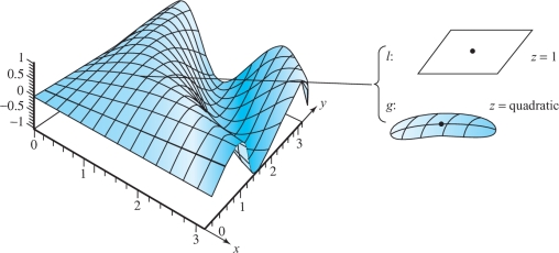
Thus, the linear (first-order) approximation is \begin{eqnarray*} l(x,y)&=&f(x_0,y_0)+f_x(x_0,y_0)(x-x_0)+f_y(x_0,y_0)(y-y_0)\\ &=& 1+0+0=1, \end{eqnarray*} and the second-order (or quadratic) approximation is \begin{eqnarray*} g(x,y) &=& 1+0+0+\frac{1}{2}\bigg({-}\frac{\pi^2}{4}\bigg)(x-1)^2+\bigg({-}\frac{\pi}{2}\bigg) (x-1)\bigg(y-\frac{\pi}{2}\bigg)\\[4pt] &&+\,\frac{1}{2}(-1)\bigg(y-\frac{\pi}{2}\bigg)^2\\[4pt] &=&1-\frac{\pi^2}{8}(x-1)^2-\frac{\pi}{2}(x-1)\bigg(y-\frac{\pi}{2}\bigg) - \frac{1}{2}\bigg(y-\frac{\pi}{2}\bigg)^2. \end{eqnarray*}
See Figure 3.5.
example 4
Find linear and quadratic approximations to the expression \((3.98\,{-}\,1)^2/(5.97\,{-}\,3)^2\). Compare with the exact value.
165
solution Let \(f(x,y)=(x-1)^2/(y-3)^2\). The desired expression is close to \(f(4,6)=1\). To find the approximations, we differentiate: \begin{eqnarray*} \displaystyle f_x&=&\frac{2(x-1)}{(y-3)^2},\qquad f_y=\frac{-2(x-1)^2}{(y-3)^3}\\[3pt] \displaystyle f_{xy}=f_{yx}&=&\frac{-4(x-1)}{(y-3)^3},\qquad f_{xx}=\frac{2}{(y-3)^2}, \qquad f_{yy}=\frac{6(x-1)^2}{(y-3)^4}. \end{eqnarray*}
At the point of approximation, we have \[ f_x(4,6)=\frac{2}{3},\qquad f_y=-\frac{2}{3},\qquad f_{xy}=f_{yx}=-\frac{4}{9}, \qquad f_{xx}=\frac{2}{9},\qquad f_{yy}=\frac{2}{3}. \]
The linear approximation is then \[ 1+\frac{2}{3}(-0.02)-\frac{2}{3}(-0.03)=1.00666. \]
The quadratic approximation is \begin{eqnarray*} 1&+&\frac{2}{3}(-0.02)-\frac{2}{3}(-0.03)+\frac{2}{9}\frac{(-0.02)^2}{2}-\frac{4}{9}(-0.02)(-0.03)+\frac{2}{3}\frac{(-0.03)^2}{2}\\[4pt] &=& 1.00674. \end{eqnarray*}
The “exact” value using a calculator is 1.00675.