4.1 Acceleration and Newton’s Second Law
In Section 2.4 we studied the basic geometry of paths, learning how to sketch curves (the images of paths) and compute tangent lines. We also learned to think of, as the name suggests, a path as the trajectory of a particle and to regard the derivative of the path as its velocity vector. In this section we continue our study of paths, including additional topics, especially acceleration and Newton’s second law.
Differentiation of Paths
Recall that a path in \({\mathbb R}^n\) is a map \({\bf c}\) of \(\,{\mathbb R}\) or an interval in \({\mathbb R}\) to \({\mathbb R}^n\). If the path is differentiable, its derivative at each time \(t\) is an \(n\times 1\) matrix. Specifically, if \(x_1(t),\ldots ,x_n(t)\) are the component functions of \({\bf c}\), the derivative matrix is \[ {\bf c}'(t)= \left[ \begin{array}{c} d x_1/{\it dt}\\ d x_2/{\it dt}\\[1pt] \vdots\\[1pt] d x_n/ {\it dt} \end{array} \right], \] which can also be written in vector form as \[ (d x_1/{\it dt},\ldots ,dx_n/{\it dt})\qquad\hbox{or as}\qquad (x'_1(t),\ldots ,x'_n(t)). \]
218
Recall from Section 2.4 that \({\bf c}'(t)\) is the tangent vector to the path at the point \({\bf c}(t)\). Also recall that if \({\bf c}\) represents the path of a moving particle, then its velocity vector is \[ {\bf v}={\bf c}'(t), \] and its speed is \(s=\|{\bf v}\|\).
The differentiation of paths is facilitated by the following rules.
Differentiation Rules
Let \({\bf b}(t)\) and \({\bf c}(t)\) be differentiable paths in \({\mathbb R}^3\) and \(p(t)\) and \(q(t)\) be differentiable scalar functions: \[ \begin{array}{r@{\quad}l} {\it Sum Rule}\,\colon &{\displaystyle \frac{d}{{\it dt}}}[{\bf b}(t)+{\bf c}(t)] ={\bf b}'(t)+{\bf c}'(t)\\[15pt] {\it Scalar Multiplication Rule}\,\colon &{\displaystyle\frac{d}{{\it dt}}}[p(t){\bf c}(t)]=p'(t){\bf c} (t)+p(t){\bf c}'(t)\\[15pt] {\it Dot Product Rule}\,\colon & {\displaystyle\frac{d}{{\it dt}}}[{\bf b}(t)\,{\cdot}\, {\bf c}(t)]={\bf b}'(t)\,{\cdot}\, {\bf c}(t)+ {\bf b}(t)\,{\cdot}\,{\bf c}'(t)\\[15pt] {\it Cross Product Rule}\,\colon &{\displaystyle\frac{d}{{\it dt}}}[{\bf b}(t)\times {\bf c}(t)]={\bf b}'(t)\times {\bf c}(t)+{\bf b}(t)\times {\bf c}'(t) \\[15pt] {\it Chain Rule}\,\colon &{\displaystyle\frac{d}{{\it dt}}}[{\bf c}(q(t))]=q'(t){\bf c}'(q(t)) \end{array} \]
These rules follow by applying the usual differentiation rules to the components.
example 1
Show that if \({\bf c}(t)\) is a vector function such that \(\|{\bf c}(t)\|\) is constant, then \({\bf c}'(t)\) is perpendicular to \({\bf c}(t)\) for all \(t\).
solution Because \(\|{\bf c}(t)\|\) is constant, so is its square \(\|{\bf c}(t)\|^2 = {\bf c}(t)\,{\cdot}\, {\bf c}(t)\). The derivative of this constant is zero, so by the dot product rule, \[ 0=\frac{d}{{\it dt}}[{\bf c}(t)\,{\cdot}\, {\bf c}(t)]={\bf c}'(t)\,{\cdot}\, {\bf c}(t)+{\bf c}(t) \,{\cdot}\,{\bf c}'(t)=2{\bf c}(t)\,{\cdot}\, {\bf c}'(t); \] thus, \({\bf c}(t)\,{\cdot}\, {\bf c}'(t)=0\); that is, \({\bf c}'(t)\) is perpendicular to \({\bf c}(t)\).
For a path describing uniform rectilinear motion, the velocity vector is constant. In general, the velocity vector is a vector function \({\bf v}={\bf c}'(t)\) that depends on \(t\). The derivative \({\bf a}=d{\bf v}/{\it dt}={\bf c}''(t)\) is called the acceleration of the curve. If the curve is \((x(t),y(t),z(t))\), then the acceleration at time \(t\) is given by \[ {\bf a}(t)=x''(t){\bf i}+y''(t){\bf j}+z''(t){\bf k} \]
example 2
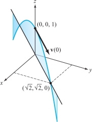
A particle moves in such a way that its acceleration is constantly equal to \(-{\bf k}\). If the position when \(t=0\) is (0, 0, 1) and the velocity at \(t=0\) is \({\bf i}+{\bf j}\), when and where does the particle fall below the plane \(z=0\)? Describe the path traveled by the particle (assume \(t\geq 0\)).
219
solution Let \(\textbf{c}(t)=(x(t),y(t),z(t))=x(t){\bf i}+y(t){\bf j}+z(t){\bf k}\) be the path traced out by the particle, so that the velocity vector is \({\bf c}'(t)=x'(t){\bf i}+y'(t){\bf j}+z'(t){\bf k}\). The acceleration \({\bf c}''(t)\) is \(-{\bf k}\), so \(x''(t)=0,y''(t)=0\), and \(z''(t)=-1\). It follows that \(x'(t)\) and \(y'(t)\) are constant functions, and \(z'(t)\) is a linear function with slope \(-1\). Because \({\bf c}'(0)={\bf i}+{\bf j}\), we get \({\bf c}'(t)={\bf i}+{\bf j}-t{\bf k}\). Integrating again and using the initial position (0, 0, 1), we find that \((x(t),y(t),z(t))= (t,t,1-\frac{1}{2}t^2)\). The particle drops below the plane \(z=0\) when \(1-\frac{1}{2}t^2=0;\) that is, \(t=\sqrt{2}\) (because \(t\ge 0\)). At that instant, the position is \((\sqrt{2},\sqrt{2},0)\). The path traveled by the particle is a parabola in the plane \(y=x\) (see Figure 4.1), because in this plane the equation is described by \(z=1-\frac{1}{2}x^2\).
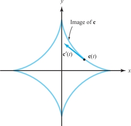
The image of a \(C^1\) path is not necessarily “very smooth”; indeed, it may have sharp bends or changes of direction. For instance, the cycloid \({\bf c}(t) = ( t - \sin t, 1- \cos t)\) shown in Figure 2.4.6 has cusps at all points where \({\bf c}\) touches the \(x\) axis (that is, when \(1-\cos t=0\), which happens when \(t=2\pi n,n=0,\pm 1,\ldots\)). Another example is the hypocycloid of four cusps, \({\bf c}\colon [0,2\pi]\rightarrow {\mathbb R}^2,t\mapsto (\,\cos^3 t,\,\sin^3 t)\), which has cusps at four points (Figure 4.2). At all such points, however, \({\bf c}'(t)={\bf 0}\), and the tangent line is not well defined. Evidently, the direction of \({\bf c}'(t)\) may change abruptly at points where it slows to rest.
A differentiable path \({\bf c}\) is said to be regular at \(t=t_{0}\) if \({\bf c}'(t_{0}) \ne {\bf 0}\). If \({\bf c}' (t) \ne {\bf 0}\) for all \(t\), we say that \(c\) is a regular path. In this case, the image curve looks smooth.
example 3
A particle moves along a hypocycloid according to the equations \[ x = \,\cos^3 t , \qquad y = \,\sin^3 t, \qquad a \le t \le b. \]
What are the velocity and speed of the particle?
solution The velocity vector of the particle is \[ {\bf v} = \frac{d x}{{\it dt}} {\bf i} + \frac{d y}{{\it dt}} {\bf j} = - ( 3 \,\sin t \,\cos^2 t) {\bf i} + ( 3 \,\cos t \,\sin^2 t) {\bf j}, \] and its speed is \[ s = \|{\bf v}\| = ( 9 \,\sin^2 t \,\cos^4 t + 9 \,\cos^2 t \,\sin^4 t)^{1/2} = 3\, |\sin t|\ \, |\!\cos t|. \]
Newton’s Second Law
220
If a particle of mass \(m\) moves in \({\mathbb R}^3\), the force \({\bf F}\) acting on it at the point \({\bf c}(t)\) is related to the acceleration \({\bf a}(t)\) by Newton’s second law:footnote # \[ {\bf F} \hbox{(}{\bf c}\hbox{(}t\hbox{)}\hbox{)} = m {\bf a}\hbox{(}t\hbox{)}. \]
In particular, if no forces act on a particle, then \({\bf a}(t)={\bf 0}\), so \({\bf c}'(t)\) is constant and the particle follows a straight line.
Acceleration and Newton’s Second Law
The acceleration of a path \({\bf c}(t)\) is \[ {\bf a}(t)={\bf c}''(t). \]
If \({\bf F}\) is the force acting and \(m\) is the mass of the particle, then \[ {\bf F}=m{\bf a}. \]
In the problem of determining the path \({\bf c}(t)\) of a particle under the influence of a given force field, \({\bf F}\), Newton’s law becomes a differential equation (i.e., an equation involving derivatives) for \({\bf c}(t)\).
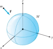
For example, the motion of a planet moving along a path \({\bf r}(t)\) around the sun (considered to be located at the origin in \({\mathbb R}^3\)) obeys the law \[ m{\bf r}”=-\frac{GmM}{r^3}{\bf r}, \] where \(M\) is the mass of the sun, \(m\) that of the planet, \(r=\|{\bf r}\|\), and \(G\) is the gravitational constant. The relation used in determining the force, \({\bf F}=-GmM{\bf r}/r^3\), is called Newton’s law of gravitation (see Figure 4.3). We shall not make a general study of such equations in this book, but content ourselves with the special case of circular orbits. (More general orbits—the conic sections—are discussed in the Internet supplement.)
Circular Orbits
Consider a particle of mass \(m\) moving at constant speed \(s\) in a circular path of radius \(r_0\). Supposing that it moves in the \(xy\) plane, we can suppress the third component and write its location as \[ {\bf r} (t) = \bigg( r_0 \,\cos \frac{st}{r_0}, r_0 \,\sin \frac{st}{r_0} \bigg). \]
221
Note that this is a circle of radius \(r_{0}\) and that its speed is given by \(\|{\bf r}{'} (t)\|=s\). The quantity \(s/r_{0}\) is called the frequency and is denoted \(\omega\). Thus, \[ {\bf r}(t) = (r_{0} \cos \, \omega t, \ r_{0} \sin \, \omega t). \]
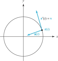
The acceleration is given by \[ {\bf a} (t) = {\bf r}'' (t) = \bigg({-} \frac{s^2}{r_0}\,\cos \frac{s t}{r_0},\, {-}\frac{s^2}{r_0} \,\sin \frac{s t}{r_0}\bigg) =\,{-}\frac{s^2}{r^2_0}{\bf r} (t) =-\omega^2{\bf r}(t). \]
Thus, the acceleration is in a direction opposite to \({\bf r} (t);\) that is, it is directed toward the center of the circle \((\)see Figure \(4.1.4)\). This acceleration multiplied by the mass of the particle is called the centripetal force. Even though the speed is constant, the direction of the velocity is continuously changing and therefore the acceleration, which is a rate of change in either speed or direction or both, is nonzero.
Newton’s law helps us discover a relationship between the radius of the orbit of a revolving body and the period; that is, the time it takes for one complete revolution. Consider a satellite of mass \(m\) moving with a speed \(s\) around a central body with mass \(M\) in a circular orbit of radius \(r_0\) (distance from the center of the spherical central body). By Newton’s second law \({\bf F}=m{\bf a}\), we get \[ -\frac{s^2 m}{r^2_0}{\bf r}(t)=-\frac{GmM}{r^3_0}{\bf r}(t). \]
The lengths of the vectors on both sides of this equation must be equal. Hence \[ s^2=\frac{{\it GM}}{r_0}. \]
If \(T\) denotes the period, then \(s=2\pi r_0/T\); substituting this value for \(s\) in the preceding equation and solving for \(T\), we obtain the following:
Kepler’s Law
\[ T^2=r^3_0\frac{(2\pi)^2}{{\it GM}}. \] Thus, the square of the period is proportional to the cube of the radius.
222
We have defined two basic concepts associated with a path: its velocity and its acceleration. Both involve differential calculus. The basic concept of the length of a path, which involves integral calculus, will be taken up in the next section.
example 4
Suppose that a satellite is to be in a circular orbit about the earth such that it stays fixed in the sky over one point on the equator. What is the radius of such a geosynchronous orbit? (The mass of the earth is \(5.98 \times 10^{24}\) kilograms and \(G=6.67 \times 10^{-11}\) in the meter-kilogram-second [kgs] system of units.)
solution The period of the satellite should be 1 day, so \(T=60\,\times\, 60 \times 24 ={86{,}400}\) seconds. From the formula \(T^2=r^3_0(2\pi)^2/{\it GM}\), we get \(r^3_0=T^2{\it GM}/(2\pi)^2\), and so \[ r^3_0 = \frac{T^2{\it GM}}{(2\pi)^2}=\frac{(86{,}400)^2\times (6.67\times 10^{-11})\times (5.98\times 10^{24})}{(2\pi)^2} \approx 7.54 \times 10^{22}\,{\rm m}^3. \]
Thus, \(r_0=4.23\times 10^7 \,{\rm m} ={42{,}300}\,{\rm km}\approx {26{,}200}\, {\rm mi.}\)
Supplement to Section 4.1: Planetary Orbits, Hamilton’s Principle, and Spacecraft Trajectories
In this section we have been studying paths in space and Newton’s second law. Hopefully, you realize that these ideas apply to the real world—the motion of our earth around the sun, for example, is governed by these laws. But there is more to the story, and we will try to convey some of it here.
Historical Note
Kepler, Newton, Hamilton, Feynman, and Planck
As we discussed in the historical introduction, the law of planetary motion stating that the square of the period is proportional to the cube of the radius of an orbit is one of the three that Kepler observed before Newton formulated his laws of motion, known more generally as Newton’s mechanics. These mechanics enable us to compute the period of a satellite about the earth or a planet about the sun (when the radius of its orbit is given), and, as we will indicate shortly, trajectories of space missions. Kepler discovered and used results like this not only for circular orbits but more generally for elliptical orbits. Newton was able to derive Kepler's three celestial laws from his own law of gravitation. The neat mathematical order of the universe that these laws provided had a great impact on eighteenth-century thought.
Newton never wrote down his laws of mechanics as differential equations. This was first done by Euler around 1730. Newton made most of his deductions (at least those in published form) by geometric methods. Euler also showed how Newton’s equations followed from Maupertuis’ action principle. The clearest version of the action principle in mechanics, now known as Hamilton’s principle, is due to William Rowan Hamilton around 1830, who, as we all should now know, happens to also be the father of vector calculus. Hamilton’s version of Maupertuis’ principle was elegantly presented by Richard Feynman, as we discuss next.
223
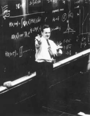
FEYNMAN AND HAMILTON’S PRINCIPLE. In his legendary Caltech Lectures on Physics, Nobel Prize–winning physicist Richard Phillips Feynman (see Figure 4.5 and Figure 4.6) included what he called a “Special Lecture” on a topic clearly very close to his heart—one that he first heard about from his New York high school teacher, Mr. Bader. Mr. Bader told his (apparently bored) student Feynman how principles of maxima and minima apply to the trajectories of moving objects and in particular how the action principle of Maupertuis, Leibniz, and Hamilton (discussed in Section 3.3) applies to Newton’s mechanics, governed by \({\bf F}\,{=}\,{\it m{\bf a}}\).
Professor Feynman, at the end of his lecture, notes that “a physicist, a student of Mr. Bader, in 1942 showed how this action principle applied to quantum mechanics.” That student was Feynman himself, who received the Nobel Prize for his insights, which also included the discovery of Feynman integrals. The moral here is pay attention to your teachers—especially the best ones!
We include the first part of Feynman’s lecture here and more of it in the Internet supplement; see Volume II, Lecture 19, of the Feynman Lectures on Physics for the entire lecture.
The Principle of Least Action, by Richard Feynman
When I was in high school, my physics teacher—whose name was Mr. Bader—called me down one day after physics class and said, “You look bored; I want to tell you something interesting.”
Then he told me something which I found absolutely fascinating, and have, since then, always found fascinating. Every time the subject comes up, I work on it. In fact, when I began to prepare this lecture I found myself making more analyses on the thing. Instead of worrying about the lecture, I got involved in a new problem. The subject is this—the principle of least action.
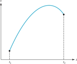
Mr. Bader told me the following: Suppose you have a particle (in a gravitational field, for instance) which starts somewhere and moves to some other point by free motion—you throw it, and it goes up and comes down [see Figure 4.7].
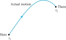
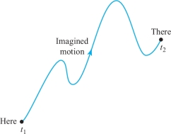
It goes from the original place to the final place in a certain amount of time. Now, you try a different motion. Suppose that to get from here to there, it went like this [see Figure 4.8], but got there in just the same amount of time.
Then he said this: “If you calculate the kinetic energy at every moment on the path, take away the potential energy, and integrate it over the time during the whole path, you’ll find that the number you’ll get is bigger than that for the actual motion.”
224
In other words, the laws of Newton could be stated not in the form \(F\,{=}\,{\it ma}\) but in the form: The average kinetic energy less the average potential energy is as little as possible for the path of an object going from one point to another.
Let me illustrate a little better what this means. If you take the case of the gravitational field, then if the particle has the path \(x\hbox{(}t\hbox{)}\) (let’s just take one dimension for a moment; we take a trajectory that goes up and down and not sideways), where \(x\) is the height above the ground, the kinetic energy is \(\textstyle\frac{1}{2}m\,\hbox{(}{\it dx}\)/\({\it dt}\,\hbox{)}^{2}\), and the potential energy at any time is mgx. Now I take the kinetic energy minus the potential energy at every moment along the path and integrate that with respect to time from the initial time to the final time. Let’s suppose that at the original time \(t_{1}\) we started at some height and at the end of the time \(t_{2}\) we are definitely ending at some other place [see Figure 4.9].
Then the integral is \[ \int^{t_2}_{t_1}\Bigg[\frac{1}{2}m\, \bigg(\frac{{\it dx}}{{\it dt}}\bigg)^2 - {\it mgx}\Bigg]\,{\it dt}. \]
225
The actual motion is some kind of curve—it’s a parabola if we plot against the time—and gives a certain value for the integral. But we could imagine some other motion that went very high and came up and down in some peculiar way [see Figure 4.10].
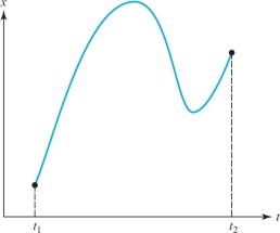
We can calculate the kinetic energy minus the potential energy and integrate for such a path . . . or for any other path we want. The miracle is that the true path is the one for which that integral is least.
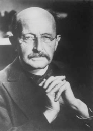
MAX PLANCK AND THE PRINCIPLE OF LEAST ACTION. Max Planck (see Figure 4.11), one of the greatest scientists of the modern era and the discoverer of the “quantization” of nature, was also a profound believer in the mathematical design of the universe, and in particular the principle of least action. He argued that the universality of this principle was evidence of a divine creator, and the structure of the universe a result of divine reason. On June 29, 1922, on “Leibniz Day” in Berlin, Germany, just a few years after World War I, with all its terrible carnage, Planck delivered an address honoring this great scholar and his discovery of the principle of least action.
In the following paragraphs we excerpt some of Planck’s remarks.
Modern science, in particular under the influence of the development of the notion of causality, has moved far away from Leibniz’s teleological point of view. Science has abandoned the assumption of a special, anticipating reason, and it considers each event in the natural and spiritual world, at least in principle, as reducible to prior states. But still we notice a fact, particularly in the most exact science, which, at least in this context, is most surprising. Present-day physics, as far as it is theoretically organized, is completely governed by a system of space–time differential equations which state that each process in nature is totally determined by the events which occur in its immediate temporal and spatial neighborhood.
This entire rich system of differential equations, though they differ in detail, since they refer to mechanical, electric, magnetic, and thermal processes, is now completely contained in a single dictum—the principle of least action. This, in short, states that, of all possible processes, the only ones that actually occur are those that involve minimum expenditure of action. As we can see, only a short step is required to recognize in the preference for the smallest quantity of action the ruling of divine reason, and thus to discover a part of Leibniz’s teleological ordering of the universe.footnote #
226
In present-day physics the principle of least action plays a relatively minor role. It does not quite fit into the framework of present theories. Of course, admittedly it is a correct statement; yet usually it serves not as the foundation of the theory, but as a true but dispensable appendix, because present theoretical physics is entirely tailored to the principle of infinitesimal local effects, and sees extensions to larger spaces and times as an unnecessary and uneconomical complication of the method of treatment. Hence, physics is inclined to view the principle of least action more as a formal and accidental curiosity than as a pillar of physical knowledge.
Real-Life Trajectories
Interesting paths in \({\mathbb R}^{3}\) that obey Newton’s second law occur in our own solar system and are used by NASA to plan space missions. One such mission, the Genesis Discovery Mission, launched from earth August 8, 2001, has a particularly interesting trajectory, as shown in Figure 4.12. More information about this trajectory and the mission objectives can be found at https://genesismission.jpl.nasa.gov/.
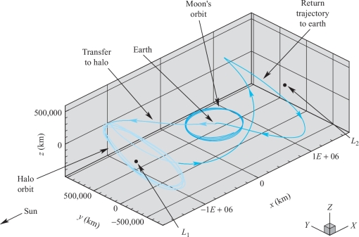
The points denoted \(L_{1}\) and \(L_{2}\) in this figure denote places of balance (discovered by Euler) between the earth and the sun. A motionless spacecraft positioned there will remain there. There are periodic orbits about these points that we have (loosely) called halo orbits. The main dynamics of the spacecraft is governed by the pull of both the earth and the sun (and to a very small extent the moon) on the spacecraft. This is thus part of the famous three-body problem studied and made famous by Poincaré around 1890.footnote #