15.4 Changing the Order of Integration
Suppose that \(D\) is a simple region—that is, it is both \(x\)-simple and \(y\)-simple. Thus, it can be given as the set of points \((x, y)\) such that \[ a\leq x\leq b, \phi_1(x)\leq y\leq \phi_2(x), \] and also as the set of points \((x, y)\) such that \[ c\leq y\leq d, \psi_1(y)\leq x\leq \psi_2(y). \]
290
Hence, we have the formulas \[ \intop\!\!\!\intop\nolimits_{D}\, f(x,y)\, {\it dA}= \int_a^b \int_{\phi_1(x)}^{\phi_2(x)} f(x,y)\, {\it dy}\,{\it dx} = \int_c^d \int_{\psi_{1}(y)}^{\psi_{2}(y)} f(x,y)\, {\it dx}\, {\it dy} . \]
If we are required to compute one of the preceding iterated integrals, we may do so by evaluating the other iterated integral; this technique is called changing the order of integration. It can be useful to make such a change when evaluating iterated integrals, because one of the iterated integrals may be more difficult to compute than the other.
example 1
By changing the order of integration, evaluate \[ \int^a_0 \int_{0}^{(a^2-x^2)^{1/2}} (a^2-y^2)^{1/2} {\it dy}\,{\it dx} . \]
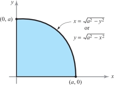
solution Note that \(x\) varies between 0 and \(a\), and for each such fixed \(x\), we have \(0\leq y\leq (a^2-x^2)^{1/2}\). Thus, the iterated integral is equivalent to the double integral \[ \intop\!\!\!\intop\nolimits_{D}\, (a^2-y^2)^{1/2} {\it dy}\,{\it dx} , \] where \(D\) is the set of points \((x, y)\) such that \(0\leq x\leq a\) and \(0\leq y\leq (a^2-x^2)^{1/2}\). But this is the representation of one-quarter (the positive quadrant portion) of the disk of radius \(a\); hence, \(D\) can also be described as the set of points \((x, y)\) satisfying \[ 0\leq y\leq a, 0\leq x\leq (a^2-y^2)^{1/2} \] (see Figure 15.28). Thus, \begin{eqnarray*} \int_0^a \int_0^{(a^2-x^2)^{1/2}} (a^2-y^2)^{1/2} {\it dy}\,{\it dx} &=& \int_0^a \bigg[ \int_0^{(a^2-y^2)^{1/2}} (a^2-y^2)^{1/2} {\it dx} \bigg]\, {\it dy}\\[4pt] &=& \int_0^a \big[x(a^2-y^2)^{1/2}\big]_{x=0}^{(a^2-y^2)^{1/2}} {\it dy} \\[4pt] &=& \int_0^a (a^2-y^2)\, {\it dy} =\bigg[a^2y-\frac{y^3}{3}\bigg]^a_0 =\frac{2a^3}{3}. \end{eqnarray*}

We could have evaluated the initial iterated integral directly, but, as you can easily verify, changing the order of integration makes the problem simpler. The next example shows that it may not be obvious how to evaluate an iterated integral, and yet it may be relatively simple to evaluate the iterated integral obtained by changing the order of integration.

291
example 2
Evaluate \[ \int_1^2 \int_0^{\log x} (x-1) \sqrt{1+e^{2y}}\ {\it dy}\, {\it dx} . \]
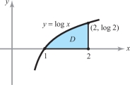
solution It will simplify matters if we first interchange the order of integration. First, notice that the integral is equal to \({\intop\!\!\!\intop}_D\, (x-1)\sqrt{1+e^{2y}}\ {\it dA}\), where \(D\) is the set of \((x, y)\) such that \[ 1\leq x\leq 2\qquad\hbox{and}\qquad 0\leq y\leq \log x. \]
The region \(D\) is simple (see Figure 15.29) and can also be described by \[ 0\leq y\leq \log 2\qquad\hbox{and}\qquad e^y\leq x\leq 2. \]
Thus, the given iterated integral is equal to \begin{equation*} \int_0^{\log 2}\int_{e^y}^2 (x-1)\sqrt{1+e^{2y}}\ {\it dx}\, {\it dy} = \int_0^{\log 2} \sqrt{1+e^{2y}}\, \bigg[ \int^2_{e^y} (x-1)\, {\it dx} \bigg]\, {\it dy}\\[4pt] \quad = \int_0^{\log 2}\sqrt{1+e^{2y}}\, \bigg[\frac{x^2}{2}-x\bigg]_{e^y}^2 {\it dy} \\[4pt] \quad = -\int_0^{\log 2}\bigg(\frac{e^{2y}}{2}-e^y\bigg)\sqrt{1+e^{2y}} {\it dy} \\[4pt] \quad = {-}\frac{1}{2}\int_0^{\log 2} e^{2y} \sqrt{1+e^{2y}} {\it dy}+ \int_0^{\log 2} e^y \sqrt{1+e^{2y}} {\it dy}.\tag{1} \end{equation*}
In the first integral in expression (1), we substitute \(u=e^{2y}\), and in the second, \(v=e^y\). Hence, we obtain \begin{equation*} -\frac{1}{4}\int_1^4 \sqrt{1+u} {\,d} u+\int_1^2 \sqrt{1+v^2} {\,d} v.\tag{2} \end{equation*}
Both integrals in expression (2) are easily found with techniques of one-variable calculus (or by consulting the table of integrals at the back of the book). For the first integral, we get \begin{equation*} \frac{1}{4}\int_1^4\sqrt{1+u} {\,d} u=\bigg[ \frac{1}{6}(1+u)^{3/2}\bigg]^4_1 = \frac{1}{6} [(1+4)^{3/2}-2^{3/2} ] = \frac{1}{6} [5^{3/2}-2^{3/2} ].\tag{3} \end{equation*}
The second integral is \begin{equation*} \begin{array}{lll} \int_1^2 \sqrt{1+v^2} {\,d} v &=& \frac{1}{2}\left[v\sqrt{1+v^2}+\log\ (\sqrt{1+v^2}+v)\right]^2_1\\[6pt] &=& \frac{1}{2}\left[2\sqrt{5}+\log\ (\sqrt{5}+2)\right]- \frac{1}{2}\left[\sqrt{2}+\log\ (\sqrt{2}+1)\right] \end{array}\tag{4} \end{equation*} (see formula 43 in the table of integrals at the back of the book). Finally, we subtract equation (3) from equation (4) to obtain the answer \[ \frac{1}{2}\bigg(2\sqrt{5}-\sqrt{2} +\log \frac{\sqrt{5}+2}{\sqrt{2}+1}\bigg) -\frac{1}{6}\big[5^{3/2}-2^{3/2}\big]. \]
Question 15.61 Section 15.5 Progress Check 1
Evaluate \[ \int \limits_0^2 \int \limits_{\frac{y}{2}}^1 e^{x^2} \ dx \ dy\]
| A. |
| B. |
| C. |
| D. |
| E. |
Mean-Value Inequality
292
We conclude with an inequality that helps us estimate integrals. Suppose there are numbers \(m\) and \(M\) such that for all \((x, y) \in D\), and \(m \leq f(x, y) \leq M\), then integrating over \(D\), we get \begin{equation*} m \,{\cdot}\, A(D) \leq \intop\!\!\!\intop\nolimits_{D} f(x, y)\, {\it dA} \leq M \,{\cdot}\, A(D),\tag{5} \end{equation*} where \(A(D)\) is the area of the region \(D\). Even though this inequality is obvious, it can help us estimate integrals that we cannot easily evaluate exactly.
example 3
Consider the integral \[ \intop\!\!\!\intop\nolimits_{D}\frac{1}{\sqrt{1+x^6+y^8}}\,{\it dx}\,{\it dy}, \] where \(D\) is the unit square \([0, 1] \times [0, 1]\). Because the integrand satisfies, for \(x\) and \(y\) between 0 and 1, \[ \frac{1}{\sqrt{3}}\leq\frac{1}{\sqrt{1+x^6+y^8}}\leq 1, \] and because the square has area 1, we get: \[ \frac{1}{\sqrt{3}}\leq\intop\!\!\!\intop\nolimits_{D}\frac{1}{\sqrt{1+x^6+y^8}}\,{\it dx}\,{\it dy}\leq 1. \]
Mean-Value Equality
The mean-value inequality can be turned into an equality when \(f\) is continuous. Here is the formal statement.
Theorem 5 Mean-Value Theorem: Double Integrals
Suppose \(f\colon D\to {\mathbb R}\) is continuous and \(D\) is an elementary region. Then for some point \((x_0, y_0)\) in \(D\) we have \[ \intop\!\!\!\intop\nolimits_{D} \, f(x,y)\, {\it dA}=f(x_0,y_0) A(D), \] where \(A(D)\) denotes the area of \(D\).
proof
We cannot prove this theorem with complete rigor, because it requires some concepts about continuous functions not proved in this course; but we can sketch the main ideas that underlie the proof.
Because \(f\) is continuous on \(D\), it has a maximum value \(M\) and a minimum value \(m\). Thus, \(m\leq f(x,y) \leq M\) for all \((x,y)\in D\). Furthermore, \(f(x_1,y_1)=m\) and \(f (x_2,y_2)=M\) for some pairs \((x_1, y_1)\) and \((x_2, y_2)\) in \(D\).
Dividing through inequality (5) by \(A(D)\), we get \begin{equation*} m\leq \frac{1}{A(D)}\intop\!\!\!\intop\nolimits_{D}\,f(x,y)\, {\it dA}\leq M.\tag{6} \end{equation*}
293
Because a continuous function on \(D\) takes on every value between its maximum and minimum values (this is the two-variable intermediate-value theorem proved in advanced calculus; see also Review Exercise 32), and because the number \([1/A(D)]{\intop\!\!\!\intop}_D f(x,y)\ {\it dA}\) is, by inequality (6), between these values, there must be a point \((x_0,y_0)\in D\) with \[ f(x_0,y_0)=\frac{1}{A(D)}\intop\!\!\!\intop\nolimits_{D}f(x,y) \,{\it dA}, \] which is precisely the conclusion of Theorem 5.
Question 15.62 Section 15.5 Progress Check Question 2
Let \(D=[0,2] \times [0,2]\) and let \(f(x,y) = x+y\). If possible, find a point \((x_0,y_0) \in D\) such that
\[ f(x_0,y_0) = \frac{1}{A(D)} \iint\limits_D f(x,y) \ dA\]
| A. |
| B. |
| C. |
| D. |
| E. |