16.4 Improper Integrals [Optional]
339
In this section, we study improper integrals—that is, integrals in which the function may be unbounded or the region of integration is unbounded. We shall first recall the situation for functions of one variable.
One-Variable Improper Integrals
In the study of integrals of functions of one variable, we encounter various types of “improper” integrals; that is, integrals of unbounded functions defined on intervals or integrals of functions over unbounded intervals. For example, \[ \int^1_0 \frac{1}{\sqrt{x}} {\it dx} \hbox{and} \int^\infty_1 \frac{{\it dx}}{x^2} \] are improper integrals. They are evaluated using a limiting process; for instance, \[ \int^1_0 \frac{1}{\sqrt{x}} {\it dx} = \lim_{a\rightarrow 0} \int^1_a \frac{1}{\sqrt{x}} {\it dx} = \lim_{a\rightarrow 0} \left(2\sqrt{x} \big|^1_a\right) = \lim_{a\rightarrow 0}\,(2-2\sqrt{a}) = 2 \] and \[ \int^\infty_1 \frac{{\it dx}}{x^2} = \lim_{b\rightarrow \infty} \int^b_1 \frac{{\it dx}}{x^2} = \lim_{b\rightarrow \infty}\left( -\frac{1}{x}\bigg|^b_1\right) = \lim_{b\rightarrow \infty} \bigg(1-\frac{1}{b}\bigg) =1. \]
If, in such a limiting process, the limit does not exist (or is infinite), we say that the integral does not exist (or that the integral diverges).
Question 16.94 Section 16.4 Progress Check Question #1
Determine if \(\displaystyle \int \limits_1^\infty x^{-\frac{4}{5}} \ dx\) converges or diverges. If the integral converges, find its value.
| A. |
| B. |
| C. |
| D. |
| E. |
Improper Integrals in the Plane
Next, we describe three types of improper integrals of two variables over a region \(D\). The first two types are described in the text below, and the third type (integrals over unbounded regions) is left to the exercises. We will evaluate all integrals using a limiting process, as in the one-variable case.
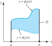
For simplicity of exposition, we first restrict ourselves to nonnegative functions \(f\)—that is, \(f(x, y) \ge 0\) for all points \((x, y) \in D\)—and to \(y\)-simple regions described as the set of \((x, y)\) such that \[ a\le x\le b, \qquad \phi_1 (x)\le y \le \phi_2 (x), \] as in Figure 16.20.
In the first case we wish to consider, let’s assume that \(f{:} \, D \rightarrow \mathbb{R}\) is continuous except for points on the boundary of \(D\). Consider, for example, \[ f(x,y) =\frac{1}{\sqrt{1-x^2-y^2}}, \] where \(D\) is the unit disk \(D= \{(x, y) | x^2 + y^2 \le 1\}\). Clearly, \(f\) is not defined on the boundary of \(D\), where \(x^2 + y^2 = 1\); yet it will be of practical interest to be able to evaluate \({\intop\!\!\intop}_D f(x, y) \, {\it dA}\), because this integral represents the area of the upper hemisphere of the unit sphere in 3-space.
Exhausting Regions
340
Our basic idea will be to integrate such an \(f\) over a smaller region \(D^\prime \), where we know the integral exists, and then let \(D^\prime\) “tend” to \(D\); that is, “exhaust” \(D\) and see if \({\intop\!\!\intop}_D f \, {\it dA}\) tends to some limit. With this in mind, we pick a special kind of \(D^\prime \), as follows.
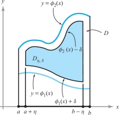
Let \(\eta > 0\) be small enough so that \(a + \eta < b\, –\, \eta\). Let \(\delta > 0\) be small enough so that \(\phi_1(x) + \delta < \phi_2(x)\, –\, \delta\) for all \(x, a \le x \le b\) (see Figure 16.21). If \(\phi_2(x) = \phi_1(x)\) for some \(x\), no such \(\delta\) will exist, but we shall worry about this minor issue when it arises in our later examples. Then the region \[ D_{\eta,\delta} = \{(x,y)| a+\eta \le x \le b - \eta \quad {\rm and}\quad \phi_1(x)+\delta \le y\le \phi_2 (x)-\delta\} \] is a subset of \(D\), and as \((\eta, \delta) \rightarrow 0, D_{\eta, \delta}\) tends to \(D\).
Improper Integrals as Limits
Because \(f\) is continuous and bounded on \(D_{\eta , \delta }\), the integral \({{\intop\!\!\!\intop}}D_{\eta , \delta } f\, {\it dA}\) exists. We can now ask what happens as the region \(D_{\eta , \delta }\) expands to fill the region, \(D\)—that is, as (\(\eta \), \(\delta ) \to\) (0, 0). Provided that \[ \lim_{(\eta,\delta)\rightarrow (0,0)}\intop\!\!\!\intop\nolimits_{D_{\eta,\delta}}f\ {\it dA} \] exists, we say that the integral of \(f\) over \(D\) is convergent or that \(f\) is integrable over \(D\), and we define \({\intop\!\!\intop}_{D} f {\it dx}\, {\it dy}\) to be equal to this limit.
example 1
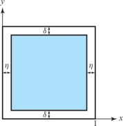
Evaluate \[ \intop\!\!\!\intop\nolimits_D \frac{1}{\root 3\of{xy}}\ {\it dA}, \] where \(D\) is the unit square [0, 1] \(\times\) [0, 1].
341
solution \(D\) is clearly a \(y\)-simple region. Choose \(\eta\) > 0 and \(\delta\) > 0 so that \(D_{\eta , \delta } \subset D\), as in Figure 16.22. Then, by Fubini’s theorem: \begin{eqnarray*} \intop\!\!\!\intop\nolimits_{D_{\eta, \delta}} \frac{1}{\root 3\of{xy}}\ {\it dA} &=& \int ^{1-\eta}_\eta \int^{1-\delta}_\delta \frac{1}{\root 3\of{xy}} {\it dy}\, {\it dx}\\[4pt] &=& \int^{1-\eta}_\eta \frac{1}{\root3\of{x}} {\it dx} \int^{1-\delta}_\delta \frac{1}{\root 3\of{y}} {\it dy}\\[4pt] &=& \frac{3}{2} \bigg((1-\eta)^{2/3}-\eta^{2/3}\bigg) \,{\cdot}\, \frac{3}{2} \bigg((1-\delta)^{2/3}-\delta^{2/3}\bigg).\\[-11pt] \end{eqnarray*}
Letting (\(\eta \), \(\delta ) \to\) (0, 0), we see that \[ \lim_{(\eta,\delta)\rightarrow (0,0)} \intop\!\!\!\intop\nolimits_{D_{\eta,\delta}} \frac{1}{\root 3\of{xy}}{\it dy}\,{\it dx} =\frac{3}{2} \frac{3}{2} = \frac{9}{4}. \]
Unfortunately, it may not always be possible to evaluate such limits so directly and simply. This is often the case in the most interesting examples, as with the surface area of the hemisphere, mentioned earlier. It’s as if the “real world” always presents the greatest challenges to the mathematician! So let us expand a bit on our theoretical discussion.
Improper Integrals as Limits of Iterated Integrals
Suppose \(f\) is integrable over \(D_{\eta , \delta }\). We can then apply Fubini’s theorem to obtain \[ \intop\!\!\!\intop\nolimits_{D_{\eta, \delta}} f\ {\it dA}= \int^{b-\eta}_{a+\eta}\int^{\phi_{ 2} (x)-\delta}_{\phi_1(x)+\delta} f (x,y)\, {\it dy}\, {\it dx}. \]
Hence, if \(f\) is integrable over \(D\), \begin{equation*} \intop\!\!\!\intop\nolimits_{D} f\ {\it dA} =\lim_{(\eta, \delta) \rightarrow (0,0)} \int^{b-\eta}_{a+\eta} \int^{\phi_2 (x)-\delta}_{\phi_1(x)+\delta} f (x,y)\, {\it dy}\, {\it dx}.\tag{1} \end{equation*}
Now \(F(\eta,\delta) = {\intop\!\!\intop}_{D_{\eta, \delta}} f\ {\it dA}\) is a function of two variables, \(\eta\) and \(\delta \), because as we change \(\eta\) and \(\delta \), we get another number. Now if \(f\) is integrable, then \[ \lim_{(\eta,\delta)\rightarrow (0,0)} F{(\eta,\delta)} =L \] exists. It follows that the iterated limits \[ \lim_{\eta\rightarrow 0}\lim_{\delta\rightarrow 0} F (\eta,\delta)\qquad \hbox{and} \qquad \lim_{\delta\rightarrow 0}\lim_{\eta\rightarrow 0} F (\eta,\delta) \] also exist and are both equal to \(L\), which in our case is \({\intop\!\!\intop}_{D} f {\it dA}\). Thus, the iterated limit \[ \lim_{\eta\rightarrow 0}\lim_{\delta\rightarrow 0} \int^{b-\eta}_{a+\eta} \int^{\phi_1 (x)-\delta}_{\phi_1 (x)+\delta} f(x,y)\, {\it dy}\, {\it dx} \] also exists. Conversely, if the iterated limits exist, it does not generally follow that the limit \(\lim_{(\eta,\delta) \rightarrow (0,0)} F(\eta,\delta)\) exists.
342
For example, if it were to turn out in some way that \(F(\eta,\delta) = {\eta\delta}/{(\eta^2+\delta^2)}\), then \(\lim_{\eta\rightarrow 0}\lim_{\delta\rightarrow 0} F(\eta,\delta) =\lim_{\delta\rightarrow 0}\lim_{\eta\rightarrow 0} F(\eta,\delta)=0\); yet \(\lim_{(\eta,\delta)\rightarrow (0,0)} F(\eta,\delta)\) does not exist, because \(F(\eta,\eta)=1/2\) (see Section 2.2).
In view of this, consider expression (1) again. If \(f\) is integrable, then \begin{eqnarray*} \intop\!\!\!\intop\nolimits_D f(x,y)\ {\it dA} &=& \lim_{(\eta,\delta)\rightarrow (0,0)} \int^{b-\eta}_{a+\eta} \int^{\phi_2 (x) -\delta}_{\phi_1 (x) +\delta} f (x,y)\, {\it dy}\, {\it dx} \\[5pt] &=& \lim_{\eta\rightarrow (0)}\lim_{\delta\rightarrow 0} \int^{b-\eta}_{a+\eta} \int^{\phi_2 (x)-\delta}_{\phi_1 (x)+\delta} f(x,y)\, {\it dy}\, {\it dx}. \end{eqnarray*}
Now suppose that for each \(x\), \[ \lim_{\delta\rightarrow 0} \int^{\phi_2 (x)-\delta}_{\phi_1 (x)+\delta} f (x,y)\, {\it dy} \] exists. Denote this by \(\int^{\phi_2(x)}_{\phi_1(x)} f(x,y)\, {\it dy}\). Suppose further that \[ \lim_{\eta\rightarrow 0} \int^{b-\eta}_{a+\eta} \int^{\phi_2 (x)}_{\phi_1(x)} f(x,y)\, {\it dy} \] also exists. We denote this limit by \(\int^b_a\int^{\phi_2 (x)}_{\phi_1(x)} f(x,y)\, {\it dy}\, {\it dx}\). Then if all limits exist, all limits must be equal. Thus, if \(f\) is integrable and the iterated improper integral exists, then necessarily \[ \intop\!\!\!\intop\nolimits_D f(x,y)\ {\it dA} = \int^b_a \int^{\phi_2(x)}_{\phi_1(x)} f(x,y)\, {\it dy}\, {\it dx}. \]
However, is it possible that the existence of just the iterated integrals implies the integrability of \(f\)? We turn to this important question next.
Fubini’s Theorem for Improper Integrals
For integrals, something truly remarkable happens. Unlike the case for iterated limits (as in the counterexample considered earlier), the existence of the iterated limits does imply the integrability of \(f\) as long as \(f \ge 0\). Thus, if \(f \ge 0\) and if \(\int^b_a \int^{\phi_2 (x)}_{\phi_1 (x)} f(x,y)\, {\it dy}\, {\it dx}\) exists as an iterated limit, then \(f\) is integrable and \[ \intop\!\!\!\intop\nolimits_{D} f(x,y)\ {\it dA} = \int^b_a \int^{\phi_2 (x)}_{\phi_1 (x)} f (x,y)\, {\it dy}\, {\it dx}. \]
If \(D\) is an \(x\)-simple region with the \(x\) coordinate lying between two functions \(\psi _{1}\) and \(\psi _{2}\), and if \[ \int^{d}_c \int^{\psi_2 ( y)}_{\psi_1 ( y)} f(x,y)\ {\it dx}\, {\it dy} \] exists as an improper integral, it again follows that \(f\) is integrable and \[ \intop\!\!\!\intop\nolimits_D f(x,y)\ {\it dA} = \int^d_c \int^{\psi_2 ( y)}_{\psi_1 ( y)} f(x, y)\ {\it dx}\, {\it dy}. \]
343
All these results, which are the improper analogues of Theorems 4 and \(4^\prime\) in Section 15.3, are known as Fubini’s theorem for improper integrals, which we formally state.
Theorem 3 Fubini’s Theorem
Let \(D\) be an elementary region in the plane and \(f \ge 0\) a function continuous except for points possibly on the boundary of \(D\). If either of the integrals \begin{eqnarray*} &\displaystyle\intop\!\!\!\intop\nolimits_D f(x,y)\ {\it dA},\\[6pt] &\displaystyle\int^b_a \int^{\phi_2(x)}_{\phi_1(x)} f(x, y)\ {\it dy}\, {\it dx}, \qquad \hbox{for }{\it y}\hbox{-simple regions}\\[6pt] & \displaystyle\int^{d}_c \int^{\psi_2 (y)}_{\psi_1(y)} f(x,y)\ {\it dx}\, {\it dy} \qquad \hbox{for }{\it x}\hbox{-simple regions} \end{eqnarray*} exist as improper integrals, \(f\) is integrable and they are all equal.
The proof of this involves advanced concepts of analysis, so we omit it here. This result can be quite useful in calculation, as the next example shows.
example 2
Let \(f(x, y) = 1/ \sqrt{1 - x^{2} - y^{2}}\) and let \(D\) be the unit disk in the plane. Show that \(f\) is integrable and that \(\smash{{\intop\!\!\intop}_{D}} f(x, y)\ {\it dA} = 2 \pi \), half the surface area of the unit sphere.
solution For \(-1 < x < 1\), we have \begin{eqnarray*} \int^{\sqrt{1-x^2}}_{-\sqrt{1-x^2}}\frac{{\it dy}}{\sqrt{1-x^2-y^2}} &=& \lim_{\delta\rightarrow 0}\int^{\sqrt{1-x^2}- \delta}_{-\sqrt{1-x^2}+\delta} \frac{{\it dy}}{\sqrt{1-x^2-y^2}}\\[5pt] &=&\lim_{\delta\rightarrow 0}\sin^{-1} \left(\frac{y}{\sqrt{1-x^2}}\right)\bigg|^{\sqrt{1-x^2}-\delta}_{-\sqrt{1-x^2}+\delta}\\[5pt] &=& \lim_{\delta\rightarrow 0}\left\{\sin^{-1}\left(1-\frac{\delta}{\sqrt{1-x^2}}\right)-\sin^{-1}\left(-1 +\frac{\delta}{\sqrt{1-x^2}}\right) \right\}\\[5pt] &=&\sin^{-1}(1) -\sin^{-1}(-1) =\frac{\pi}{2}-\frac{(-\pi)}{2} =\pi.\\[-17pt] \end{eqnarray*}
Clearly, \[ \lim_{\eta\rightarrow 0}\int^{1-\eta}_{-1+\eta} \int^{\sqrt{1-x^2}}_{-\sqrt{1-x^2}}\ \frac{{\it dy}\, {\it dx}}{\sqrt{1-x^2 -y^2}} = \lim_{\eta\rightarrow 0}\int^{1-\eta}_{-1+\eta}\ \pi {\it dx} = \lim_{\eta\rightarrow 0} \pi (2-2\eta)=2\pi. \]
Thus, \(f\) is integrable. To see why this theorem is so useful, try to show directly from the definition that \(f\) is integrable. It is not easy to do so!
Question 16.95 Section 16.4 Progress Check Question #2
Determine if \(\displaystyle \int_0^1 \int_0^1 \frac{x}{\sqrt{1-y^2}} \ dy \ dx\) converges or diverges. If the integral converges, find its value.
| A. |
| B. |
| C. |
| D. |
| E. |
example 3
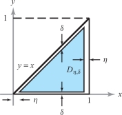
Let \(f(x, y) = 1/(x - y)\) and let \(D\) be the set of (\(x, y)\) satisfying \(0 \le x \le 1\) and \(0 \le y \le x\). Show that \(f\) is not integrable over \(D\).
solution Because the denominator of \(f\) is zero on the line \(y=x\), \(f\) is unbounded on part of the boundary of \(D\). Let \(0 < \eta < 1\) and \(0 < \delta < \eta \), and let \(D_{\eta , \delta }\) be the set of (\(x, y)\) with \(\eta \le x \le 1 - \eta\) and \(\delta \le y \le x - \delta\) (Figure 16.23).
344
Here the region \(D\) is \(y\)-simple with \(\phi _{1}(x)\) = 0, \(\phi _{2}(x)=x,\) and \(\phi _{1}\)(0) = \(\phi _{2}\)(0). To ensure that \(D_{\eta , \delta } \subset D\) and is depicted in the figure, we must choose \(\delta\) a bit more carefully. A little geometry shows that we should choose \(2\delta \leq \eta\). Consider \begin{eqnarray*} \intop\!\!\!\intop\nolimits_{D_{\eta,\delta}} f {\it dA} &=& \int^{1-\eta}_\eta \int^{x-\delta}_\delta \frac{1}{x-y} \ {\it dy}\, {\it {\,d} x}\\[5pt] &=& \int^{1-\eta}_\eta [-\log\,(x-y)] |^{x-\delta}_{y=\delta} {\it {\,d} x}\\[5pt] &=& \int^{1-\eta}_\eta [-\log\,(\delta)+ \log\,(x-\delta)] {\it {\,d} x}\\[5pt] &=& [-\log\delta] \int^{1-\eta}_\eta {\it {\,d} x} + \int^{1-\eta}_\eta \log\,(x-\delta)\, {\it {\,d} x}\\[5pt] &=& -(1-2\eta) \log \delta + [(x-\delta)\log\,(x-\delta)-(x-\delta)]|^{1-\eta}_\eta. \end{eqnarray*}
In the last step, we used the fact that \(\int \log u\ du = u \log u - u\). Continuing the preceding set of qualities, we have \begin{eqnarray*} \intop\!\!\!\intop\nolimits_{D_{\eta,\delta}} f\ {\it dA} &=& -(1-2\eta)\log\delta + (1-\eta -\delta) \log\,(1-\eta -\delta)\\ &&-1(1-\eta -\delta) - (\eta-\delta)\log\,(\eta-\delta) + (\eta -\delta). \end{eqnarray*}
As (\(\eta , \delta ) \to (0, 0)\), the second term converges to 1 log \(1 = 0\), and the third and fifth terms converge to \(-1\) and 0, respectively. Let \(v=\eta - \delta\). Because \(v\) log \(v \to 0\) as \(v \to 0\) (a limit established by using L’Hôpital’s rule from calculusfootnote #), we see that the fourth term goes to zero as (\(\eta , \delta ) \to (0, 0)\). It is the first term that will give us trouble. Now: \begin{equation*} -(1 - 2\eta ) \log \delta = - \log \delta + 2\eta \log \delta ,\tag{2} \end{equation*} and it is not hard to see that this does not converge as (\(\eta , \delta ) \to (0, 0)\). For example, let \(\eta = 2 \delta \); then expression (2) becomes \(-\log \delta + 4 \delta \log \delta\). As before, \(4\delta \log \delta \to 0\) as \(\delta \to 0\), but \(-\log \delta \to +\infty\) as \(\delta \to 0\), which shows that expression (2) does not converge. Hence, \(\lim_{(\eta,\delta) \rightarrow (0,0)} {\intop\!\!\intop}_{D_{\eta,\delta}}f\ {\it dA}\) does not exist and so \(f\) is not integrable.
Functions Unbounded at Isolated Points
We now consider nonnegative functions \(f\) that become “infinite” or are undefined at isolated points in an \(x\)-simple or \(y\)-simple region \(D\). For example, consider the function \(f(x, y) = 1/ \sqrt{x^{2}+y^{2}}\) on the unit disk \(D = \{ (x, y) \vert x^{2} + y^{2} \le 1 \}\). Again, \(f \ge 0\), but \(f\) is unbounded and is not defined at the origin.
Let \((x_{0}, y_{0})\) be a point of a general region \(D\) where a nonnegative function \(f\) is undefined. Further, let \(D_{\delta }=D_{\delta } (x_{0}, y_{0})\) be the disk of radius \(\delta\) centered at (\(x_{0}, y_{0})\) and let \(D\backslash D_{\delta }\) denote the region \(D\) with \(D_{\delta }\) removed. Assume that \(f\) is continuous at every point of \(D\) except (\(x_{0}, y_{0})\). Then \({\intop\!\!\intop}_{D\backslash D_{\delta}} f\ {\it dA}\) is defined. We say that \({\intop\!\!\intop}_{D} f\ {\it dA}\) is convergent, or that \(f\) is integrable over \(D\) if \[ \lim_{\delta\rightarrow 0} \intop\!\!\!\intop\nolimits_{D\backslash D_\delta} f\ {\it dA} \] exists.
345
example 4
Show that \(f(x, y) = 1/ \sqrt{x^{2}+y^{2}}\) is integrable over the unit disk \(D\) and evaluate \({\intop\!\!\intop}_{D} f {\it dA}\).
solution Let \(D_{\delta }\) be the disk of radius \(\delta\) centered at the origin. Then \(f\) is continuous everywhere on \(D\) except at (0, 0). Thus, \({\intop\!\!\intop}_{D\backslash D_\delta} f\ {\it dA}\) exists. To evaluate this integral, we change variables to polar coordinates, \(x=r \cos \theta, y=r \sin \theta\). Then \(f (r \cos \theta , r \sin \theta ) = 1/ r\), and \[ \intop\!\!\!\intop\nolimits_{D\backslash D_\delta} f \,{\it dA} = \int^1_\delta \int^{2\pi}_0 \frac{1}{r} r\ d\theta\ dr = \int ^1_\delta\int^{2\pi}_0 d\theta\ dr = 2\pi (1-\delta). \] Thus, \[ \intop\!\!\!\intop\nolimits_{D} f\ {\it dA} = \lim_{\delta\rightarrow 0} \intop\!\!\!\intop\nolimits_{D\backslash D_\delta} f\ {\it dA} = 2\pi. \]
More generally, we can, in an analogous manner, define the integral of nonnegative functions \(f\) that are continuous except at a finite number of points in \(D\). We can also combine both types of improper integrals; that is, we may consider functions that are continuous except at a finite number of points on \(D\) or at points on the boundary of \(D\), and define \({\intop\!\!\intop}_{D} f\ {\it dA}\) appropriately.
If \(f\) takes both positive and negative values, we can use a more advanced integration theory, called the Lebesgue integral, to generalize the notion of convergent integral \({\intop\!\!\intop}_{D}\) f dA. Using this theory, it is possible to show that if \({\intop\!\!\intop}_{D} f\ {\it dA}\) exists, it can then be evaluated as an iterated integral. This latter fact is also known as Fubini’s theorem.
Unbounded Regions
As was mentioned previously, we will leave consideration of unbounded regions to the exercise section. However, we must point out that we have already addressed the main idea in Example 5 of Section 16.2 on the Gaussian integral. In that example, we integrated \(\hbox{exp}(-x^{2} - y^{2})\) over all of \({\mathbb{R}}^{2}\) by integrating first over a disk of radius \(a\) and then letting \(a \to \infty\).