17.1 The Path Integral
This section introduces the concept of a path integral; this is one of the several ways in which integrals of functions of one variable can be generalized to functions of several variables. Besides those in Chapter 15, there are other generalizations, to be discussed in later sections.
Suppose we are given a scalar function \(f\colon \,{\mathbb R}^3 \rightarrow {\mathbb R}\), so that \(f\) sends points in \({\mathbb R}^3\) to real numbers. It will be useful to define the integral of such a function \(f\) along a path \({\bf c} \colon I = [a,b] \rightarrow {\mathbb R}^3\), where \({\bf c}(t) = (x(t), y(t), z(t))\). To relate this notion to something tangible, suppose that the image of \({\bf c}\) represents a wire. We can let \(f(x,y,z)\) denote the mass density at \((x, y, z)\) and the integral of \(f\) will be the total mass of the wire. By letting \(f(x, y, z)\) indicate temperature, we can also use the integral to determine the average temperature along the wire. We first give the formal definition of the path integral and then, after the following example, further motivate it.
352
Definition: Path Integrals
The path integral, or the integral of \(f(x, y, z)\) along the path \({\bf c}\), is defined when \({\bf c}\colon I=[a,b] \rightarrow {\mathbb R}^3\) is of class \(C^1\) and when the composite function \(t \mapsto f(x(t),y(t), z(t))\) is continuous on \(I\). We define this integral by the equation \[ \int_{\bf c} f \,{\it ds} = \int_a^b f(x(t),y(t), z(t)) \| {\bf c}'(t) \| \,{\it dt}. \]
Sometimes \(\int_{\tiny \bf c} f \,{\it ds}\) is denoted \[ \int_{\bf c} f(x,y,z) \,{\it ds} \] or \[ \int^b_a f({\bf c}(t))\| {\bf c}' (t)\| \,{\it dt} . \]
If \({\bf c}(t)\) is only piecewise \(C^1\) or \(f({\bf c}(t))\) is piecewise continuous, we define \(\int_{\bf c}f \,{\it ds}\) by breaking \([a,b]\) into pieces over which \(f({\bf c}(t))\| {\bf c}' (t)\|\) is continuous, and summing the integrals over the pieces.
When \(f=1\), we recover the definition of the arc length of \({\bf c}\). Also note that \(f\) need only be defined on the image curve \(C\) of \({\bf c}\) and not necessarily on the whole space in order for the preceding definition to make sense.
example 1
Let \({\bf c}\) be the helix \({\bf c}\colon \,[0,2\pi] \rightarrow {\mathbb R}^3, t \mapsto (\cos t,\sin t,t)\) (see Figure 2.4.9), and let \(f(x,y,z)= x^2 + y^2 + z^2\). Evaluate the integral \(\int_{\bf c}f(x,y,z)\,{\it ds}\).
solution First we compute \(\| {\bf c}' (t)\|\): \[ \| {\bf c}' (t)\| = \sqrt{\bigg[ \frac{d(\cos t)}{{\it dt}}\bigg]^2 +\bigg[ \frac{d(\sin t)}{{\it dt}}\bigg]^2 + \bigg[ \frac{{\it dt}}{{\it dt}}\bigg]^2}= \sqrt{\sin^2 t + \cos^2 t + 1} = \sqrt{2}. \]
Next, we substitute for \(x\), \(y\), and \(z\) in terms of \(t\) to obtain \[ f(x,y,z) = x^2 + y^2 + z^2 = \cos^2 t + \sin^2 t + t^2 = 1 + t^2 \] along \({\bf c}\). Inserting this information into the definition of the path integral yields \[ \int_{\bf c}f(x,y,z)\,{\it ds} = \int_0^{2\pi} (1 + t^2) \sqrt{2}\,{\it dt}= \sqrt{2}\, \bigg[t + \frac{t^3}{3}\bigg]_0^{2\pi} = \frac{2\sqrt{2}\pi}{3} (3 + 4\pi^2). \]
353
To motivate the definition of the path integral, we shall consider “Riemann-like” sums \(S_N\) in the same general way we did to define arc length in Section 12.3. For simplicity, let \({\bf c}\) be of class \(C^1\) on \(I\). Subdivide the interval \(I=[a,b]\) by means of a partition \[ a=t_0 < t_1 < \cdots < t_N = b. \]
This leads to a decomposition of \({\bf c}\) into paths \({\bf c}_i\) (Figure 17.1) defined on \([t_i,t_{i+1}]\) for \(0 \leq i \leq N -1\). Denote the arc length of \({\bf c}_i\) by \({\Delta} s_i \); thus, \[ {\Delta} s_i = \int^{t_{i+1}}_{t_i} \| {\bf c}'(t)\| \,{\it dt}. \]
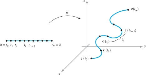
When \(N\) is large, the arc length \({\Delta} s_i\) is small and \(f(x,y,z)\) is approximately constant for points on \({\bf c}_i\). We consider the sums \[ S_N = \sum_{i=0}^{N-1} f(x_i,y_i,z_i)\, {\Delta} s_i , \] where \((x_i,y_i,z_i)={\bf c}(t)\) for some \(t \in [t_i, t_{i+1}]\). By the mean-value theorem we know that \(\Delta s_i =\|{\bf c}'(t_i^*)\| \Delta t_i\), where \(t_i \leq t_i^* \leq t_{i+1}\) and \(\Delta t_i = t_{i + 1}- t_i\). From the theory of Riemann sums, it can be shown that \begin{eqnarray*} {\displaystyle \mathop {\rm limit}_{N \rightarrow \infty}\ } S_N = {\displaystyle \mathop {\rm limit}_{N \rightarrow \infty}\ } \sum^{N-1}_{i=0} f(x_i,y_i,z_i) \|{\bf c}'(t_i^*)\| \Delta t_i &=& \int_I f(x(t),y(t), z(t)) \| {\bf c}'(t) \| \,{\it dt}\\[3pt] &=& \int_{\bf c} f(x,y,z) \,{\it ds}. \end{eqnarray*}
Question 17.1 Section 17.1 Progress Check Question #1
Evaluate the path integral \(\int_{\bf c} xy \ ds\) where \({\bf c}:[0,\frac{\pi}{2}] \longrightarrow \mathbb{R}^3\) is given by \({\bf c}(t) = (\cos t, \sin t, \cos t) \).
| A. |
| B. |
| C. |
| D. |
| E. |
| F. |
| G. |
The Path Integral for Planar Curves
An important special case of the path integral occurs when the path \({\bf c}\) describes a plane curve. Suppose that all points \({\bf c}(t)\) lie in the \({\it xy}\) plane and \(f\) is a real-valued function of two variables. The path integral of \(f\) along \({\bf c}\) is \[ \int_{\bf c} f(x,y)\,{\it ds} = \int^b_a f(x(t),y(t)) {\sqrt{x'(t)^2 + y'(t)^2}} \,{\it dt} . \]
354
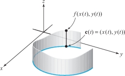
When \(f(x, y) \geq 0\), this integral has a geometric interpretation as the “area of a fence.” We can construct a “fence” with base the image of \({\bf c}\) and with height \(f(x, y)\) at \((x, y)\) (Figure 17.2). If \({\bf c}\) moves only once along the image of \({\bf c}\), the integral \(\int_{\bf c}f(x,y)\,{\it ds}\) represents the area of a side of this fence. Readers should try to justify this interpretation for themselves, using an argument like the one used to justify the arc-length formula.
example 2
Tom Sawyer’s aunt has asked him to whitewash both sides of the old fence shown in Figure 17.3. Tom estimates that for each \(25 {\rm ft}^2\) of whitewashing he lets someone do for him, the willing victim will pay 5 cents. How much can Tom hope to earn, assuming his aunt will provide whitewash free of charge?
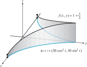
solution From Figure 17.3, the base of the fence in the first quadrant is the path \({\bf c}\colon \, [0,\pi/2]\rightarrow {\mathbb R}^2, t \mapsto (30 \cos^3 t , 30 \sin^3 t)\), and the height of the fence at \((x, y)\) is \(f(x,y) = 1 + y/3\). The area of one side of the half of the fence is equal to the integral \(\int_{\bf c}f(x,y)\,{\it ds} =\int_{\bf c}(1+y/3) \,{\it ds}\). Because \({\bf c}'(t)=(-90 \cos^2 t \sin t, 90 \sin^2 t \cos t)\), we have \(\| {\bf c}'(t) \| = 90 \sin t \cos t\). Thus, the integral is \begin{eqnarray*} \int_{\bf c}\bigg( 1 + \frac{y}{3} \bigg)\, {\it ds} &=& \int_0^{\pi/2} \bigg(1 + \frac{30 \sin^3 t}{3}\bigg) 90 \sin t \cos t \,{\it dt} \\[9pt] &=& 90 \int_0^{\pi/2} (\sin t + 10 \sin^4 t) \cos t \,{\it dt} \\[9pt] &=& 90 \bigg[ \frac{\sin^2 t}{2} + 2 \sin^5 t\bigg]^{\pi/2}_0= 90 \bigg(\frac{1}{2} + 2\bigg)=225, \end{eqnarray*} which is the area in the first quadrant. Hence, the area of one side of the fence is \(450 {\rm ft}^2\). Because both sides are to be whitewashed, we must multiply by 2 to find the total area, which is \(900 {\rm ft}^2\). Dividing by 25 and then multiplying by 5, we find that Tom could realize as much as $1.80 for the job.
Question 17.2 Section 17.1 Progress Check Question #2
Evaluate the path integral \(\int_{\bf c} (x^2-y) \ ds\) where \({\bf c}:[0,1] \longrightarrow \mathbb{R}^2\) is given by \({\bf c}(t) = (3t, 4t) \).
This concludes our study of integration of scalar functions over paths. In the next section we shall turn our attention to the integration of vector fields over paths, and we shall see many further applications of the path integral in Chapter 18, when we study vector analysis.
Supplement to Section 17.1: The Total Curvature of a Curve
Exercises 16, 17, and 20–23 of Section 12.3 described the notions of curvature \(\kappa\) and torsion \(\tau\) of a smooth curve \(C\) in space. If \({\bf c}: [a, b] \to C \ {\subset} \ {\mathbb R}^{3}\) is a unit-speed parametrization of \(C\), so that \(\| {\bf c}'(t)\| = 1\), then the curvature \(\kappa(p)\) at \(p \in C\) is defined by \(\kappa (p)=\| {\bf c}''(t)\|\), where \(p = {\bf c}(t)\). A result of differential geometry is that two unit-speed curves with the same curvature and torsion can be obtained from one another by a rigid rotation, translation, or reflection.
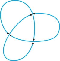
The curvature \(\kappa{:}\, C \to {\mathbb R}\) is a real-valued function on the set \(C\), so we define the total curvature as its path integral over \(C\): \(\int_{C} \kappa\,{\it ds}\). There are some surprising facts that mathematicians have been able to prove about the total curvature. For one thing, if \(C\) is a closed [that is, \({\bf c}(a) ={\bf c}(b)\)] planar curve, then \[ \int _{C} \kappa \,{\it ds} \ge 2\pi \] and equals 2\(\pi\) only when \(C\) is a circle. If \(C\) is a closed space curve with \[ \int _{C} \kappa \,{\it ds} \le 4\pi, \] then \(C\) is “unknotted”; that is, \(C\) can be continuously deformed (without ever intersecting itself) into a planar circle. Therefore, for knotted curves, \[ \int _{C} \kappa\, {\it ds} > 4\pi. \]
See Figure 17.4.
356
The formal statement of this fact is known as the Fary–Milnor theorem. Legend has it that John Milnor, a contemporary of John Nash'sfootnote # at Princeton University, was asleep in a math class as the professor wrote three unsolved knot theory problems on the blackboard. At the end of the class, Milnor (still an undergraduate) woke up and, thinking the blackboard problems were assigned as homework, quickly wrote them down. The following week he turned in the solution to all three problems—one of which was a proof of the Fary–Milnor theorem! Some years later, he was appointed a professor at Princeton, and in 1962 he was awarded (albeit for other work) a Fields medal, mathematics’ highest honor, generally regarded as the mathematical Nobel Prize.