18.1 Green’s Theorem
428
Green’s theorem relates a line integral along a closed curve \(C\) in the plane \({\mathbb R}^2\) to a double integral over the region enclosed by \(C\). This important result will be generalized in the following sections to curves and surfaces in \({\mathbb R}^3\). We shall be referring to line integrals around curves that are the boundaries of elementary regions (see Section 5.3). To understand the ideas in this section, you may also need to refer to Section 7.2.
Simple and Elementary Regions and Their Boundaries
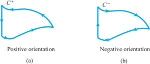
A simple closed curve \(C\) that is the boundary of an elementary region has two orientations—counterclockwise (positive) and clockwise (negative). We denote \(C\) with the counterclockwise orientation as \(C^{+}\), and with the clockwise orientation as \(C^{-}\) (Figure 18.1).
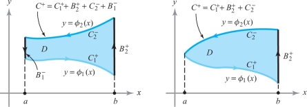
The boundary \(C\) of a \(y\)-simple region can be decomposed into bottom and top portions, \(C_1\) and \(C_2\), and (if applicable) left and right vertical portions, \(B_1\) and \(B_2\). Following Figure 18.2, we write, \[ C^{+} = C^{+}_1 + B^{+}_2 + C^{-}_2 + B^{-}_1, \] where the pluses denote the curves oriented in the direction of left to right or bottom to top, and the minuses denote the curves oriented from right to left or from top to bottom.
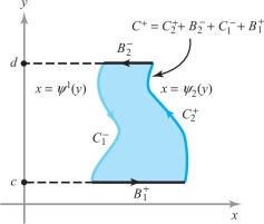
We can make a similar decomposition of the boundary of an \(x\)-simple region into left and right portions, and upper and lower horizontal portions (if applicable) (Figure 18.3).
Similarly, the boundary of a simple region has two decompositions: one into upper and lower halves, the other into left and right halves.
Green’s Theorem
429
We shall now prove two lemmas in preparation for Green’s theorem.
Lemma 1
Let \(D\) be a \(y\)-simple region and let \(C\) be its boundary. Suppose \(P \colon\, D \to {\mathbb R}\) is of class \(C^1\). Then \[ \int_{C^+} P {\,d} x = - \intop\!\!\!\intop\nolimits_{D} \frac{\partial\! P}{\partial y} {\it {\,d} x}\, {\it dy}. \] (The left-hand side denotes the line integral \(\int_{C^+} P {\it {\,d} x} + Q\, {\it dy}\), where \(Q = 0\).)
proof
Suppose \(D\) is described by \[ a \le x \le b \qquad \phi_1 (x) \le y \le \phi_2 (x). \]
We decompose \(C^+\) by writing \(C^{+} = C^{+}_1 \,+\, B_2^{+} \,+\, C_2^{-} \,+\, B_1^{-}\) (see Figure 18.2). By Fubini’s theorem, we can evaluate the double integral as an iterated integral and then use the fundamental theorem of calculus: \begin{eqnarray*} \intop\!\!\!\intop\nolimits_{D} \frac{\partial\! P}{\partial y} (x,y) {\it {\,d} x}\, {\it dy} & = & \int_a^b \int_{\phi_1(x)}^{\phi_2 (x)} \frac{\partial\! P}{\partial y} (x,y)\, {\it dy}\, {\it {\,d} x}\\[8pt] & = & \int_a^b [P (x, \phi_2(x)) -P (x, \phi_1 (x)) ] {\it {\,d} x}. \end{eqnarray*}
However, because \(C_1^{+}\) can be parametrized by \(x \mapsto (x, \phi_1(x)), a\le x \le b\), and \(C_2^{+}\) can be parametrized by \(x \mapsto (x, \phi_2 (x)), a\le x \le b\), we have \[ \int_a^b P (x, \phi_1 (x)) {\it {\,d} x} = \int_{C_1^{+}} P (x,y) {\it {\,d} x} \] and \[ \int_a^bP(x,\phi_2(x))\,{\it {\,d} x}=\int_{C_{2}^{+}}P(x,y)\,{\it {\,d} x}. \]
430
Thus, by reversing orientations, \[ - \int_a^b P (x, \phi_2 (x)) {\it {\,d} x} = \int_{C_2^{-}} P (x,y) {\it {\,d} x}. \]
Hence, \[ \intop\!\!\!\intop\nolimits_{D} \frac{\partial\! P}{\partial y} {\it {\,d} x}\, {\it dy} = - \int_{C_1^{+}} P {\it {\,d} x} - \int_{C_2^{-}} P {\it {\,d} x}. \]
Because \(x\) is constant on \(B_2^{+}\) and \(B_1^{-}\), we have \[ \int_{B_2^{+}} P {\it {\,d} x}=0 = \int_{B_1^{-}} P {\it {\,d} x}, \] so \[ \int_{C^{+}} P {\it {\,d} x} = \int_{C^{+}_1} P {\it {\,d} x}+ \int_{B^{+}_2} P {\it {\,d} x} + \int_{C_2^{-}} P {\it {\,d} x} + \int_{B_1^{-}} P {\it {\,d} x} = \int_{C_1^{+}} P {\it {\,d} x} + \int_{C_2^{-}} P {\it {\,d} x}. \]
Thus, \[ \intop\!\!\!\intop\nolimits_{D} \frac{\partial\! P}{\partial y} {\it {\,d} x}\, {\it dy} = - \int_{C_1^{+}} P {\it {\,d} x} - \int_{C_2^{-}} P {\it {\,d} x} = - \int_{C^{+}} P {\it {\,d} x}. \]
We now prove the analogous lemma with the roles of \(x\) and \(y\) interchanged.
Lemma 2
Let \(D\) be an \(x\)-simple region with boundary \(C\). Then if \(Q\colon\, D \to {\mathbb R}\) is \(C^1\), \[ \int_{C^{+}} Q \,{\it dy} = \intop\!\!\!\intop\nolimits_{D} \frac{\partial\! Q}{\partial x} {\it {\,d} x}\, {\it dy}. \]
The negative sign does not occur here, because reversing the role of \(x\) and \(y\) corresponds to a change of orientation for the plane.
proof
Suppose \(D\) is given by \[ \psi_1 (y) \le x \le \psi_2 (y), c \le y \le d. \]
Using the notation of Figure 18.3, and noting that \(y\) is constant on \(B^+_1\) and \(B^-_2\), we have \[ \int_{C^{+}} Q \,{\it dy} = \int_{C_1^{-} +B_1^{+} + C_2^{+} + B_2^{-}} Q \,{\it dy} = \int_{C_2^{+}} Q \,{\it dy} + \int_{C_1^-} Q \,{\it dy}, \] where \(C_2^{+}\) is the curve parametrized by \(y \mapsto (\psi_2 (y), y), c \le y \le d\), and \(C_1^{+}\) is the curve \(y \mapsto ( \psi_1 (y), y), c \le y \le d\). Applying Fubini’s theorem and the fundamental theorem of calculus, we obtain \begin{eqnarray*} \intop\!\!\!\intop\nolimits_{D} \frac{\partial\! Q}{\partial x} {\it {\,d} x}\, {\it dy} &=& \int_c^d \int_{\psi_1 (y)}^{\psi_2 (y)} \frac{\partial\! Q}{\partial x} {\it {\,d} x}\,{\it dy} = \int_c^d [ Q (\psi_2 (y),y) - Q (\psi_1 (y), y)]\, {\it dy}\\[6pt] & = & \int_{C_2^{+}} Q \,{\it dy} - \int_{C_1^{+}} Q \,{\it dy} = \int_{C^{+}_2} Q \,{\it dy} + \int_{C^{-}_1} Q \,{\it dy} = \int_{C^{+}} Q \,{\it dy}.\\[-25pt] \end{eqnarray*}
431
Adding the results of Lemmas 1 and 2 proves the following important theorem.
Theorem 1 Green’s Theorem
Let \(D\) be a simple region and let \(C\) be its boundary. Suppose \(P \colon\, D \to {\mathbb R}\) and \(Q\colon\, D \to {\mathbb R}\) are of class \(C^1\). Then \[ \int_{C^{+}} P {\it {\,d} x} + Q \,{\it dy} = \intop\!\!\!\intop\nolimits_{D} \left( \frac{\partial\! Q}{\partial x} - \frac{\partial\! P}{\partial y} \right) {\it {\,d} x}\, {\it dy}. \]
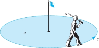
The correct (positive) orientation for the boundary curves of region \(D\) can be remembered by the following device: If you walk along the curve C with the correct orientation, the region D will be on your left (see Figure 18.4).
Historical Note
George Green
George Green was born in Nottingham England in 1793 and died in 1841. No picture of him is known to exist. Little is known about his early life before the age of 30 other than that he was a self-taught man, who developed a passion for mathematics at an early age. In 1833, at age 40, Green enrolled as a student in Cambridge. Amazingly, five years earlier, he had published (at his own expense) his first and most famous work “An Essay on the Application of Mathematical Analysis to the Theories of Electricity and Magnetism.” Here he proved a theorem similar to the Green’s Theorem of this section and also introduced other very important mathematical concepts such as Green’s functions, now so ubiquitous in mathematical analysis. He was the first person to create a theory of electricity and magnetism, a theory that later formed the basis of the work of Maxwell and others.
Generalizing Green’s Theorem
432
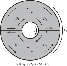
Green’s theorem actually applies to any “decent” region in \({\mathbb R}^2\). For instance, Green’s theorem applies to regions that are not simple, but that can be broken up into pieces, each of which is simple. An example is shown in Figure 18.5. The region \(D\) is an annulus; its boundary consists of two curves \(C = C_1 + C_2\) with the indicated orientations. (Note that for the inner region the correct orientation to ensure the validity of Green’s theorem is clockwise; the device in Figure 18.4 still works for remembering the orientation!) If Theorem 1 is applied to each of the regions \(D_1, D_2, D_3\), and \(D_4\) and the results are summed, the equality of Green’s theorem will be obtained for \(D\) and its boundary curve \(C\). This works because the integrals along the interior lines in opposite directions cancel. This trick, in fact, shows that Green’s theorem holds for virtually all regions with reasonable boundaries that one is likely to encounter (see Exercise 16).
Let us use the notation \(\partial\! D\) for the oriented curve \(C^{+}\), that is, the boundary curve of \(D\) oriented in the sense as described by the device in Figure 18.4. Then we can write Green’s theorem as \[ \int_{\partial\! D} P {\it {\,d} x} + Q \,{\it dy} = \intop\!\!\!\intop\nolimits_{D} \left( \frac{\partial\! Q}{\partial x} - \frac{\partial\! P}{\partial y} \right)\!\! {\it {\,d} x}\, {\it dy}. \]
Green’s theorem is very useful because it relates a line integral around the boundary of a region to an area integral over the interior of the region, and in many cases it is easier to evaluate the line integral than the area integral or vice versa. For example, if we know that \(P\) vanishes on the boundary, we can immediately conclude that \({\intop\!\!\!\intop}_D ( \partial\! P / \partial y) {\it {\,d} x}\, {\it dy} =0\) even though \(\partial\! P / \partial y\) need not vanish on the interior. (Can you construct such a \(P\) on the unit square?)
example 1
Verify Green’s theorem for \(P (x,y) =x\) and \(Q(x,y)=xy\), where \(D\) is the unit disc \(x^2 + y^2 \le 1\).
solution We do this by evaluating both sides in Green’s theorem directly. The boundary of \(D\) is the unit circle parametrized by \(x =\cos t, y = \sin t, 0 \le t \le 2 \pi\), and so \begin{eqnarray*} \int_{\partial\! D} P {\it {\,d} x} + Q\, {\it dy} & = & \int_0^{2 \pi} [( \cos t) ({-}\!\sin t) + \cos t \sin t \cos t] {\it {\,d} t} \\[6pt] & = & \left[\frac{\cos^2 t}{2} \right]_0^{2 \pi}+ \left[ - \frac{\cos^3 t}{3} \right]_0^{2 \pi} =0. \end{eqnarray*}
433
On the other hand, \[ \intop\!\!\!\intop\nolimits_{D}\left( \frac{\partial\! Q}{\partial x} - \frac{\partial\! P}{\partial y}\right) {\it dx}\, {\it dy} = \intop\!\!\!\intop\nolimits_{D} y {\it {\,d} x}\, {\it dy}, \] which is also zero by symmetry. Thus, Green’s theorem is verified in this case.
Question 18.1 Section 18.1 Progress Check Question #1
Let \(D\) be the unit disk and let \({\bf c}(t) = (\cos t, \sin t), 0 \leq t \leq 2 \pi\). According to Green's theorem, which of the following statements is true?
| A. |
| B. |
| C. |
| D. |
| D. |
Areas
We can use Green’s theorem to obtain a formula for the area of a region bounded by a simple closed curve.
Theorem 2 Area of a Region
If \(C\) is a simple closed curve that bounds a region to which Green’s theorem applies, then the area of the region \(D\) bounded by \(C = \partial\! D\) is \[ A = \frac{1}{2} \int_{\partial\! D} x {\it dy} - y {\it {\,d} x}. \]
proof
Let \(P (x,y) = - y, Q (x,y) =x\); then by Green’s theorem we have \begin{eqnarray*} \frac{1}{2} \int_{\partial\! D} x {\it dy} \,-\, y {\it {\,d} x} &=& \frac{1}{2} \intop\!\!\!\intop\nolimits_{D} \left[ \frac{\partial x}{\partial x} - \frac{\partial (-y)}{\partial y} \right] {\it dx}\, {\it dy} \\ [6pt] &=& \frac{1}{2} \intop\!\!\!\intop\nolimits_{D} [1\,+\,1] {\it {\,d} x}\, {\it dy} = \intop\!\!\!\intop\nolimits_{D} {\it {\,d} x}\, {\it dy} =A. \\[-35pt] \end{eqnarray*}
example 2
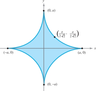
Let \(a > 0\). Compute the area (see Figure 18.6) of the region enclosed by the hypocycloid defined by \(x^{2/3} + y^{2/3} = a^{2/3}\) using the parametrization \[ x =a \cos^3 \theta , y =a \sin^3 \theta , 0 \le \theta \le 2 \pi. \]
434
solution From the preceding box, and using the trigonometric identities \(\cos^2\theta+\sin^2\theta=1, \sin 2\theta=2\sin\theta\cos\theta\), and \(\sin^2\phi=(1-\cos2\phi)/2\), we get \begin{eqnarray*} A & = & \frac{1}{2} \int_{\partial\! D} x {\it dy} - y {\it {\,d} x} \\[8pt] & = & \frac{1}{2} \int_0^{2 \pi} [(a \cos^3 \theta) ( 3 a \sin^2 \theta \cos \theta) - ( a \sin^3 \theta)(-3 a \cos^2 \theta\sin \theta) ] {\,d} \theta \\[8pt] & = & \frac{3}{2} a^2 \int_0^{2 \pi} ( \sin^2 \theta \cos^4 \theta + \cos^2 \theta \sin^4 \theta) {\,d} \theta = \frac{3}{2} a^2 \int_0^{2 \pi} \sin^2 \theta \cos^2 \theta {\,d} \theta \\[8pt] & = & \frac{3}{8} a^2 \int_0^{2 \pi} \sin^2 2 \theta {\,d} \theta = \frac{3}{8} a^2 \int_0^{2 \pi} \left( \frac{1 - \cos\, 4 \theta}{2} \right) d \theta \\[8pt] & = & \frac{3}{16} a^2 \int_0^{2 \pi} {\,d} \theta - \frac{3}{16} a^2 \int_0^{2 \pi} \cos 4 \theta {\,d} \theta = \frac{3}{8} \pi a^2.\\[-28pt] \end{eqnarray*}
Question 18.2 Section 18.1 Progress Check Question #2
Let \(C\) be the boundary of the unit square \([0,1] \times [0,1]\), oriented counter-clockwise. Find \(\displaystyle \int_{C} x {\it dy} - y {\it dx}\)
Vector Form Using the Curl
The statement of Green’s theorem can be neatly rewritten in the language of vector fields. As we will see, this points the way to one possible generalization to \({\mathbb R}^3\).
Theorem 3 Vector Form of Green’s Theorem
Let \(D \subset {\mathbb R}^2\) be a region to which Green’s theorem applies, let \(\partial\! D\) be its (positively oriented) boundary, and let \({\bf F} = P {\bf i} + Q {\bf j}\) be a \(C^1\) vector field on \(D\). Then \[ \int_{\partial\! D} {\bf F} \,{\cdot}\, d {\bf s}= \intop\!\!\!\intop\nolimits_{D} ({\rm curl}\, {\bf F}) \,{\cdot}\, {\bf k}\, {\it {\,d} A} = \intop\!\!\!\intop\nolimits_{D} ( {\nabla} \times {\bf F}) \,{\cdot}\, {\bf k}\, {\it {\,d} A} \] (see Figure 18.7).
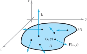
This result follows from Theorem 1 and the fact that \((\nabla\times {\bf F})\,{\cdot}\,{\bf k}=\partial\! Q/\partial x-\partial\! P/\partial y\). We ask you to supply the details in Exercise 22.
435
example 3
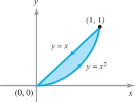
Let \({\bf F} = ( xy^2 , y+ x)\). Integrate \(({\nabla} \times {\bf F}) \,{\cdot}\, {\bf k}\) over the region in the first quadrant bounded by the curves \(y = x^2\) and \(y=x\).
solution Method 1. We first compute the curl \[ {\nabla} \times {\bf F} = \left(0, 0, \frac{\partial\! F_2}{\partial x} -\frac{\partial\! F_1}{\partial y} \right) = (1- 2 xy) {\bf k}. \]
Thus, \(({ \nabla} \times {\bf F} ) \,{\cdot}\, {\bf k} = 1 - 2 xy\). This can be integrated over the given region \(D\) (see Figure 18.8) using an iterated integral as follows: \begin{eqnarray*} \intop\!\!\!\intop\nolimits_{D} ({\nabla} \times {\bf F}) \,{\cdot}\,{\bf k} {\it {\,d} x}\, {\it dy} &=& \int_0^1 \int_{x^2}^x (1-2xy)\, {\it dy}\, {\it {\,d} x} = \int_0^1 [y-xy^2]|_{x^2}^x {\it {\,d} x} \\[6pt] & = & \int_0^1 [x - x^3 - x^2 + x^5] {\it {\,d} x} = \frac{1}{2} - \frac{1}{4} - \frac{1}{3} + \frac{1}{6} = \frac{1}{12}. \end{eqnarray*}
Method 2. Here we use Theorem 3 to obtain \[ \intop\!\!\!\intop\nolimits_{D} ( {\nabla} \times {\bf F} ) \,{\cdot}\, {\bf k} {\it {\,d} x}\, {\it dy} = \int_{\partial\! D} {\bf F} \,{\cdot}\,d {\bf s}. \]
The line integral of \({\bf F}\) along the curve \(y=x\) from left to right is \[ \int_0^1 F_1 {\it {\,d} x} + F_2\, {\it dy} = \int_0^1 ( x^3+ 2x)\, {\it {\,d} x} = \frac{1}{4}+1 = \frac{5}{4}. \]
Along the curve \(y = x^2\) we get \[ \int_0^1 F_1 {\it {\,d} x} + F_2\, {\it dy} = \int_0^1 x^5 {\it {\,d} x} + ( x+ x^2) (2 x {\it {\,d} x}) = \frac{1}{6} + \frac{2}{3} + \frac{1}{2} = \frac{4}{3}. \]
Thus, remembering that the integral along \(y=x\) is to be taken from right to left, as in Figure 18.8, \[ \int_{\partial\! D} {\bf F} \,{\cdot}\, d {\bf s} = \frac{4}{3} - \frac{5}{4} = \frac{1}{12}. \]
Vector Form Using the Divergence
436
There is another form of Green’s theorem that can be generalized to \({\mathbb R}^3\).
Theorem 4 Divergence Theorem in the Plane
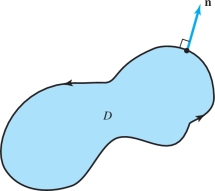
Let \(D \subset {\mathbb R}^2\) be a region to which Green’s theorem applies and let \(\partial\! D\) be its boundary. Let \({\bf n}\) denote the outward unit normal to \(\partial\! D\). If \({\bf c} \colon\, [a,b] \to {\mathbb R}^2 , t \mapsto {\bf c} (t) = (x(t) , y(t))\) is a positively oriented parametrization of \(\partial\! D, {\bf n}\) is given by \[ {\bf n} = \frac{(y' (t), - x' (t))}{\sqrt{[x' (t) ]^2 + [y' (t) ]^2}} \] (see Figure 18.9). Let \({\bf F} = P {\bf i}+ Q {\bf j}\) be a \(C^1\) vector field on \(D\). Then \[ \int_{\partial\! D} {\bf F} \,{\cdot}\, {\bf n} {\,d} s = \intop\!\!\!\intop\nolimits_{D} {\rm div\ } {\bf F}\, {\,d}\! A. \]
proof
Recall that \({\bf c}' (t) = ( x' (t), y' (t))\) is tangent to \(\partial\! D\), and note that \({\bf n} \,{\cdot}\, {\bf c}' =0\). Thus, \({\bf n}\) is normal to the boundary. The sign of \({\bf n}\) is chosen to make it correspond to the outward (rather than the inward) direction. By the definition of the line integral (see Section 7.2), \begin{eqnarray*} \int_{\partial\! D} {\bf F} \,{\cdot} {\bf n}\, ds & = & \int_a^b \frac{P (x(t), y(t)) y' (t) - Q (x(t), y(t)) x'(t)}{\sqrt{[x' (t)]^2+ [y' (t) ]^2}} {\textstyle \sqrt{[x'(t)]^2 + [y' (t) ]^2}}\, {\it {\,d} t} \\[6pt] & = & \int_a^b [P (x (t), y(t)) y' (t) - Q(x(t), y(t)) x' (t)]\, {\it {\,d} t} \\[6pt] & =& \int_{\partial\! D} P {\it dy} - Q {\it {\,d} x}. \end{eqnarray*}
By Green’s theorem, this equals \[ \intop\!\!\!\intop\nolimits_{D} \left( \frac{\partial\! P}{\partial x}+ \frac{\partial\! Q}{\partial y} \right) {\it dx}\, {\it dy} = \intop\!\!\!\intop\nolimits_{D} \hbox{div } {\bf F} {\it {\,d} A}. \]
437
example 4
Let \({\bf F} = y^3 {\bf i} + x^5 {\bf j}\). Compute the integral of the normal component of \({\bf F}\) around the unit square.
solution This can be done using the divergence theorem. Indeed \[ \int_{\partial\! D} {\bf F} \,{\cdot}\, {\bf n}\, ds = \intop\!\!\!\intop\nolimits_{D} \hbox{div } {\bf F} {\it {\,d} A}. \]
But div \({\bf F}=0\), and so the integral is zero.
Question 18.3 Section 18.1 Progress Check Question #3
Let \(C\) be the positively oriented perimeter of the rectangle \([1,3] \times [2,3]\). Find \(\displaystyle \int_{C} (3x^4+5) {\it dx} +(y^5+3y^2-1) {\it dy}\)