18.2 Stokes’ Theorem
Stokes’ theorem relates the line integral of a vector field around a simple closed curve \(C\) in \({\mathbb R}^3\) to an integral over a surface \(S\) for which \(C\) is the boundary. In this regard it is very much like Green’s theorem.
Stokes’ Theorem for Graphs
Let us begin by recalling a few facts from Chapter 17. Consider a surface \(S\) that is the graph of a function \(f (x,y)\), so that \(S\) is parametrized by \[ \left\{ \begin{array}{l} x=u \\ y=v \\ z = f (u,v) = f (x,y) \end{array}\right. \] for \((u,v)\) in some domain \(D\) in the plane. The integral of a vector function \({\bf F}\) over \(S\) was developed in Section 7.6 as \begin{equation} \intop\!\!\!\intop\nolimits_{S} {\bf F} \,{\cdot}\, d {\bf S} = \intop\!\!\!\intop\nolimits_{D} \left[ F_1 \left( - \frac{\partial z}{\partial x} \right)+ F_2 \left( - \frac{\partial z}{\partial y} \right)+ F_3 \right] {\it dx}\, {\it dy}, \end{equation} where \({\bf F} = F_1 {\bf i}+ F_2 {\bf j}+ F_3 {\bf k}\).
440
In Section 18.1, we first assumed that the regions \(D\) under consideration were simple; while this was used in our proof of Green’s theorem, we noted there that the theorem is valid for a wider class of regions. In this section we assume that \(D\) is a region whose boundary is a simple closed curve and to which Green’s theorem applies. Green’s theorem involves choosing an orientation on the boundary of \(D\), as was explained in Section 18.1. The choice of orientation that validates Green’s theorem will be called positive. Recall that if \(D\) is simple, then the positive orientation is the counterclockwise one.
Suppose that \({\bf c} \colon\, [a,b] \to {\mathbb R}^2, {\bf c} (t) = (x (t), y(t))\) is a parametrization of \(\partial\! D\) in the positive direction. Then we define the boundary curve \(\partial\! S\) to be the oriented simple closed curve that is the image of the mapping \({\bf p} \colon\, t \mapsto (x(t), y(t), f (x(t), y(t)))\) with the orientation induced by \({\bf p}\) (Figure 18.11).
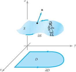
To remember this orientation (i.e., the positive direction) on \(\partial\! S\), imagine that you are an “observer” walking along the boundary of the surface with the normal as your upright direction; you are moving in the positive direction if the surface is on your left. This orientation on \(\partial\! S\) is often called the orientation induced by an upward normal \({\bf n}\).
Theorem 5 Stokes’ Theorem for Graphs
Let \(S\) be the oriented surface defined by a \(C^2\) function \(z = f(x,y)\), where \((x,y) \in D\), a region to which Green’s theorem applies, and let \({\bf F}\) be a \(C^1\) vector field on \(S\). Then if \(\partial\! S\) denotes the oriented boundary curve of \(S\) as just defined, we have \[ \intop\!\!\!\intop\nolimits_{S} \hbox{curl }{\bf F} \,{\cdot}\, d {\bf S} = \intop\!\!\!\intop\nolimits_{S} ({\nabla} \times {\bf F}) \,{\cdot}\, d {\bf S} = \int_{\partial S} {\bf F} \,{\cdot}\, d {\bf s}. \]
Remember that \(\int_{\partial S} {\bf F} \,{\cdot}\,d {\bf s}\) is the integral around \(\partial\! S\) of the tangential component of \({\bf F}\), while \({\intop\!\!\!\intop}_S {\bf G} \,{\cdot}\, d {\bf S}\) is the integral over \(S\) of \({\bf G} \,{\cdot}\, {\bf n}\), the normal component of \({\bf G}\) (see Sections 7.2 and 7.6). Thus, Stokes’ theorem says that the integral of the normal component of the curl of a vector field \({\bf F}\) over a surface \(S\) is equal to the integral of the tangential component of \({\bf F}\) around the boundary \(\partial\! S\).
441
proof
If \({\bf F} = F_1 {\bf i} + F_2 {\bf j}+ F_3 {\bf k}\), then \[ \hbox{curl } {\bf F}= \left(\frac{\partial\! F_3}{\partial\! y} - \frac{\partial\! F_2}{\partial z} \right) {\bf i} + \left(\frac{\partial\! F_1}{\partial z} - \frac{\partial\! F_3}{\partial x} \right) {\bf j} + \left(\frac{\partial\! F_2}{\partial x} - \frac{\partial\! F_1}{\partial\! y} \right) {\bf k} . \]
Therefore, we use formula (1) to write \begin{equation} \begin{array}{lll} \intop\!\!\!\intop\nolimits_{S}{\rm curl\ }{\bf F}\,{\cdot}\, d{\bf S}&=&\intop\!\!\!\intop\nolimits_{D}\bigg[ \left(\frac{\partial\! F_3}{\partial\! y}-\frac{\partial\! F_2}{\partial z}\right) \left(-\frac{\partial z}{\partial x}\right)\\[6pt] && + \left(\frac{\partial\! F_1}{\partial z}-\frac{\partial\! F_3}{\partial x} \right) \left(-\frac{\partial z}{\partial\! y}\right)+\left(\frac{\partial\! F_2}{\partial x}-\frac{\partial\! F_1}{\partial\! y}\right)\bigg]\, {\it dA}. \end{array} \end{equation}
On the other hand, \[ \int_{\partial\! S} {\bf F} \,{\cdot}\, d {\bf s} = \int_{\bf p} {\bf F} \,{\cdot}\, d{\bf s}\,=\, \int_{\bf p} F_1 {\it {\,d} x} + F_2\, {\it dy} + F_3 {\,d} z, \] where \({\bf p} \colon\, [a,b] \to {\mathbb R}^3, {\bf p} (t) = (x(t), y(t), f(x(t), y(t)))\) is the orientation-preserving parametrization of the oriented simple closed curve \(\partial\! S\) discussed earlier. Thus, \begin{equation} \int_{\partial\! S} {\bf F} \,{\cdot}\, d {\bf s} = \int_a^b \left( F_1\, \frac{{\it dx}}{{\it dt}}+ F_2\, \frac{{\it dy}}{{\it dt}} + F_3\, \frac{dz}{{\it dt}} \right) {\it dt}. \end{equation}
By the chain rule, \[ \frac{dz}{{\it dt}} = \frac{\partial z}{\partial x} \frac{d x}{d t} + \frac{\partial z}{\partial\! y} \frac{d y}{d t}. \]
Substituting this expression into equation (3), we obtain \begin{equation} \begin{array}{lll} \int_{\partial\! S} {\bf F} \,{\cdot}\, d {\bf s} & = & \int_a^b \left[ \left( F_1 + F_3 \,\frac{\partial z}{\partial x} \right) \frac{d x}{d t} + \left( F_2 + F_3\, \frac{\partial z}{\partial\! y} \right) \frac{d y}{d t} \right] {\it dt} \\[6pt] & = & \int_{\bf c} \left( F_1 + F_3 \,\frac{\partial z}{\partial x} \right) {\it dx} + \left( F_2 + F_3\, \frac{\partial z}{\partial\! y} \right) {\it dy} \\[6pt] & = & \int_{\partial\! D} \left( F_1 + F_3 \,\frac{\partial z}{\partial x} \right) {\it dx} + \left( F_2 + F_3 \,\frac{\partial z}{\partial\! y} \right) {\it dy}. \end{array} \end{equation}
Applying Green’s theorem to equation (4) yields (we are assuming that Green’s theorem applies to \(D\)) \[ \intop\!\!\!\intop\nolimits_{D} \left[ \frac{\partial ( F_2 + F_3\, \partial z / \partial\! y)}{\partial x} - \frac{\partial (F_1 + F_3 \,\partial z/ \partial x)}{\partial\! y} \right] {\it dA}. \]
Now we use the chain rule, remembering that \(F_1, F_2\), and \(F_3\) are functions of \(x,y\), and \(z\) and that \(z\) is a function of \(x\) and \(y\), to obtain \begin{eqnarray*} && \intop\!\!\!\intop\nolimits_{D} \bigg[ \left( \frac{\partial\! F_2}{\partial x}+ \frac{\partial\! F_2}{\partial z} \frac{\partial z}{\partial x}+ \frac{\partial\! F_3}{\partial x}\frac{\partial z}{\partial y}+ \frac{\partial\! F_3}{\partial z}\frac{\partial z}{\partial x}\frac{\partial z}{\partial y}+ F_3 \,\frac{\partial^2 z}{\partial x \partial y} \right) \\[6pt] && - \left( \frac{\partial\! F_1}{\partial y}+ \frac{\partial\! F_1}{\partial z}\frac{\partial z}{\partial y}+ \frac{\partial\! F_3}{\partial y}\frac{\partial z}{\partial x}+ \frac{\partial\! F_3}{\partial z}\frac{\partial z}{\partial y}\frac{\partial z}{\partial x}+ F_3\, \frac{\partial^2 z}{\partial y\, \partial x} \right)\bigg]\, {\it dA}. \end{eqnarray*}
Because mixed partials are equal, the last two terms in each parenthesis cancel each other, and we can rearrange terms to obtain the integral of equation (2), which completes the proof.
442
example 1
Let \({\bf F} = ye^{z} {\bf i}+ xe^{z} {\bf j} + xy e^{z} {\bf k}\). Show that the integral of \(\,{\bf F}\) around an oriented simple closed curve \(C\) that is the boundary of a surface \(S\) is 0. (Assume \(S\) is the graph of a function, as in Theorem 5.)
solution Indeed, \(\int_C {\bf F} \,{\cdot}\, d {\bf s} = {\intop\!\!\!\intop}_S\, ( {\nabla} \times {\bf F}) \,{\cdot}\,d {\bf S}\), by Stokes’ theorem. But we compute \[ {\nabla} \times {\bf F} = \left| \begin{array}{c@{\quad}c@{\quad}c} \displaystyle {\bf i} & {\bf j} & {\bf k} \\[5pt] \displaystyle \frac{\partial\!}{\partial x} & \displaystyle\frac{\partial\!}{\partial y} & \displaystyle \frac{\partial\!}{\partial z} \\[5pt] \displaystyle y e^{z} & x e^{z} & x y e^{z} \end{array} \right| = {\bf 0}, \] and so \(\int_C {\bf F} \,{\cdot}\, d {\bf s} =0\). Alternatively, we can observe that \({\bf F} = {\nabla} (xye^{z})\), so its integral around a closed curve is zero.
example 2
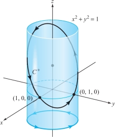
Use Stokes’ theorem to evaluate the line integral \[ \int_C - y^3 {\it {\,d} x}+x^3 {\it dy} - z^3 {\,d} z, \] where \(C\) is the intersection of the cylinder \(x^2 + y^2=1\) and the plane \(x+ y + z=1\), and the orientation on \(C\) corresponds to counterclockwise motion in the \(xy\) plane.
solution The curve \(C\) bounds the surface \(S\) defined by the equation \(z= 1-x-y=f(x,y)\) for \((x, y)\) in the set \(D = \{(x,y) \mid x^2 + y^2 \le 1\}\) (Figure 18.12). We set \({\bf F} = - y^3 {\bf i} + x^3 {\bf j} - z^3 {\bf k}\), which has curl \({ \nabla} \times {\bf F} = ( 3x^2 + 3 y^2) {\bf k}\). Then, by Stokes’ theorem, the line integral is equal to the surface integral \[ \intop\!\!\!\intop\nolimits_{S} ( {\nabla} \times {\bf F}) \,{\cdot}\, d {\bf S}. \]
But \({ \nabla} \times {\bf F}\) has only a \({\bf k}\) component. Thus, by formula (1) we have \[ \intop\!\!\!\intop\nolimits_{S}( {\nabla} \times {\bf F}) \,{\cdot}\,d {\bf S}=\intop\!\!\!\intop\nolimits_{D}(3x^2+3y^2)\,{\it {\,d} x}\,{\it dy}. \]
443
This integral can be evaluated by changing to polar coordinates. Doing this, we get \[ 3 \intop\!\!\!\intop\nolimits_{D} (x^2 + y^2)\, {\it {\,d} x}\,{\it dy} =3 \int_0^1 \int_0^{2 \pi} r^2 \,{\cdot}\, r {\,d} \theta {\,d} r = 6 \pi \int_0^1 r^3 {\,d} r = \frac{6 \pi}{4} = \frac{3 \pi}{2}. \]
Let us verify this result by directly evaluating the line integral \[ \int_C - y^3 {\it {\,d} x}+ x^3 \,{\it dy}- z^3 {\,d} z. \]
We can parametrize the curve \(\partial\! D\) by the equations \[ x = \cos t , \qquad y = \sin t,\qquad z=0, \qquad 0 \le t \le 2 \pi. \]
The curve \(C\) is therefore parametrized by the equations \[ x = \cos t, \qquad y = \sin t, \qquad z =1-\sin t - \cos t, \qquad 0 \le t \le 2 \pi. \]
Thus, \begin{eqnarray*} && \int_C \,-\, y^3 {\it {\,d} x} + x^3 {\it dy} - z^3 {\,d} z \\[2pt] &&\quad = \int_0^{2 \pi}[(-\sin^3 t) ( -\sin t) + ( \cos^3 t) ( \cos t) \\[5pt] &&\qquad{-}\,( 1-\sin t -\cos t)^3 (-\cos t + \sin t)]\, {\it {\,d} t} \\[5pt] &&\quad = \int_0^{2 \pi} ( \cos^4 t + \sin^4 t) \,{\it {\,d} t} - \int_0^{2 \pi} ( 1-\sin t -\cos t)^3 ( -\cos t + \sin t) \,{\it {\,d} t}.\\[-12pt] \end{eqnarray*}
The second integrand is of the form \(u^3 {\,d} u\), where \(u=1 -\sin t - \cos t\), and thus the integral is equal to \[ {\displaystyle \frac{1}{4}} [(1 - \sin t - \cos t)^4 ]^{2 \pi}_0=0. \]
Hence, we are left with \[ \int_0^{2 \pi} ( \cos^4 t+ \sin^4 t ) \,{\it {\,d} t}. \]
This integral can be evaluated using formulas (18) and (19) of the table of integrals. We can also proceed as follows. Using the trigonometric identities \[ \sin^2 t= \frac{1- \cos 2t}{2}, \cos^2 t = \frac{1 + \cos 2 t}{2}, \] substituting and squaring these expressions, we reduce the preceding integral to \[ \frac{1}{2} \int_0^{2 \pi}( 1+ \cos^2 2t)\,{\it {\,d} t} = \pi + \frac{1}{2} \int_0^{2 \pi}\cos^2 2 t \,{\it {\,d} t}. \]
Again using the identity \(\cos^2 2 t = (1+ \cos 4t)/2\), we find \begin{eqnarray*} \pi + \frac{1}{4}\int_0^{2 \pi}( 1+ \cos 4t) \,{\it {\,d} t} &= & \pi + \frac{1}{4} \int_0^{2 \pi}\,{\it {\,d} t} + \frac{1}{4}\int_0^{2 \pi}\cos\, 4t \,{\it {\,d} t} \\[6pt] & = & \pi + \frac{\pi}{2}+ 0 = \frac{3 \pi}{2}. \\[-32pt] \end{eqnarray*}
Question 18.42 Section 18.2 Progress Check Question #1
Use Stokes’ theorem to evaluate the line integral \[ \int_C - e^{z^2} {\it {\,d} x}+ {\it dy} - 2xze^{z^2} {\,d} z, \] where \(C\) is the boundary of the triangle with vertices (0,0,0), (0,2,0) and (0,0,3), oriented by that order.
Stokes’ Theorem for Parametrized Surfaces
444
To simplify the proof of Stokes’ theorem given earlier, we assumed that the surface \(S\) could be described as the graph of a function \(z = f (x,y), (x,y) \in D\), where \(D\) is some region to which Green’s theorem applies. However, without too much more effort we can obtain a more general theorem for oriented parametrized surfaces \(S\). The main complication is in the definition of \(\partial\! S\).
Suppose \({\Phi} \colon\, D \to {\mathbb R}^3\) is a parametrization of a surface \(S\) and \({\bf c} (t) = ( u (t) , v (t))\) is a parametrization of \(\partial\! D\). We might be tempted to define \(\partial\! S\) as the curve parametrized by \(t \mapsto {\bf p} (t) = {\Phi} ( u (t), v (t))\). However, with this definition, \(\partial\! S\) might not be the boundary of \(S\) in any reasonable geometric sense.
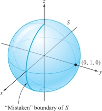
For example, we would conclude that the boundary of the unit sphere \(S\) parametrized by spherical coordinates in \({\mathbb R}^3\) is half of the great circle on \(S\) lying in the \(xz\) plane, but clearly in a geometric sense \(S\) is a smooth surface (no points or cusps) with no boundary or edge at all (see Figure 18.13 and Exercise 20). Thus, this great circle is in some sense the “mistaken” boundary of \(S\).
We can get around this difficulty by assuming that \({\Phi}\) is one-to-one on all of \(D\). Then the image of \(\partial\! D\) under \({\Phi}\), namely, \({\Phi} ( \partial\! D)\), will be the geometric boundary of \(S = {\Phi} (D)\). If \({\bf c} (t) = (u (t), v (t))\) is a parametrization of \(\partial\! D\) in the positive direction, we define \(\partial\! S\) to be the oriented simple closed curve that is the image of the mapping \({\bf p}\colon\, t \mapsto {\Phi} ( u (t), v (t))\), with the orientation of \(\partial\! S\) induced by \({\bf p}\) (see Figure 18.11).
Theorem 6 Stokes’ Theorem: Parametrized Surfaces
Let \(S\) be an oriented surface defined by a one-to-one parametrization \({\Phi}\colon\, D \subset {\mathbb R}^2 \to S\), where \(D\) is a region to which Green’s theorem applies. Let \(\partial\! S\) denote the oriented boundary of \(S\) and let \({\bf F}\) be a \(C^1\) vector field on \(S\). Then \[ \intop\!\!\!\intop\nolimits_{S}\ ( {\nabla} \times {\bf F} ) \,{\cdot}\, d {\bf S} = \int_{\partial\! S} {\bf F} \,{\cdot}\, d{\bf s}. \]
If \(S\) has no boundary, and this includes surfaces such as the sphere, then the integral on the left is zero (see Exercise 25).
This is proved in the same way as Theorem 5.
example 3
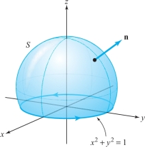
Let \(S\) be the surface shown in Figure 18.14, with the indicated orientation. Let \({\bf F} = y {\bf i} - x {\bf j} + e^{xz} {\bf k}\). Evaluate \({\intop\!\!\!\intop}_S\ ( { \nabla} \times {\bf F}) \,{\cdot}\, d {\bf S}\).
445
solution This surface could be parametrized using spherical coordinates based at the center of the sphere. However, we need not explicitly find \({\Phi}\) in order to solve this problem. By Theorem 6, \({\intop\!\!\!\intop}_S\ ( {\nabla} \times {\bf F}) \,{\cdot}\, d {\bf S}= \int_{\partial\! S}{\bf F}{\cdot} {\,d} {\bf s}\), and so if we parametrize \(\partial\! S\) by \(x (t) = \cos t, y (t) = \sin t , 0 \le t \le 2 \pi\), we determine \[ \int_{\partial\! S}{\bf F} \,{\cdot}\,d {\bf s} = \int_0^{2 \pi} \Big( y \frac{{\it dx}}{{\it dt}}- x \frac{{\it dy}}{{\it dt}} \Big)\, {\it dt} = \int_0^{2 \pi} ( - \sin^2 t- \cos^2 t) \,{\it {\,d} t} = - \int_0^{2 \pi}\,{\it {\,d} t} =- 2 \pi \] and therefore \({\intop\!\!\!\intop}_S\ ({\nabla} \times {\bf F}) \,{\cdot}\, d {\bf S} = - 2 \pi\).
Question 18.43 Section 18.2 Progress Check Question #2
Let \(S\) be the portion of the cone \(\displaystyle z= \sqrt{x^2+y^2}\) where \(z \leq 4\), oriented with the upward normal. Find the flux of the curl of \({\bf F}(x,y,z) = (yz,-xz,xy)\) across \(S\). Note: the surface \(S\) does not include the lid at the top, i.e. the surface \(S\) is not closed.
| A. |
| B. |
| C. |
| D. |
| E. |
| F. |
| G. |
The Curl as Circulation per Unit Area
Let us now use Stokes’ theorem to justify the physical interpretation of \({\nabla} \times {\bf F}\) in terms of paddle wheels that was proposed in Chapter 13. Paraphrasing Theorem 6, we have \[ \intop\!\!\!\intop\nolimits_{S} (\hbox{curl } {\bf F}) \,{\cdot}\, {\bf n}\, {\it {\,d} S} = \intop\!\!\!\intop\nolimits_{S} (\hbox{curl } {\bf F}) \,{\cdot}\, {\,d} {\bf S} = \int_{\partial\! S} {\bf F} \,{\cdot}\, {\,d} {\bf s} = \int_{\partial\! S} F_T {\,d} s, \] where \(F_T\) is the tangential component of \({\bf F}\). This says that the integral of the normal component of the curl of a vector field over an oriented surface \(S\) is equal to the line integral of \({\bf F}\) along \(\partial\! S\), which in turn is equal to the path integral of the tangential component of \({\bf F}\) over \(\partial\! S\).
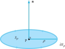
Suppose \({\bf V}\) represents the velocity vector field of a fluid. Consider a point P and a unit vector \({\bf n}\). Let \(S_\rho\) denote the disc of radius \(\rho\) and center P, which is perpendicular to \({\bf n}\). By Stokes’ theorem, \[ \intop\!\!\!\intop\nolimits_{{S_\rho}} \hbox{curl } {\bf V} \,{\cdot}\, d {\bf S} = \intop\!\!\!\intop\nolimits_{S_\rho} \hbox{curl } {\bf V} \,{\cdot}\, {\bf n}\,{\it {\,d} S} = \int_{\partial\! S_\rho} {\bf V} \,{\cdot}\, d {\bf s}, \] where \(\partial\! S_\rho\) has the orientation induced by \({\bf n}\) (see Figure 18.15).
By the mean-value theorem for integrals (Exercise 16, Section 7.6), there is a point Q in \(S_\rho\) such that \[ \intop\!\!\!\intop\nolimits_{{S_\rho}} \hbox{curl } {\bf V} \,{\cdot}\, {\bf n} {\,d} S = [ \hbox{curl }{\bf V} ({\rm Q}) \,{\cdot}\, {\bf n} ] A ( S_\rho), \] where \(A(S_\rho)=\pi \rho^2\) is the area of \(S_\rho\) and curl \({\bf V} ({\rm Q})\) is the value of curl \({\bf V}\) at Q. Thus, \begin{eqnarray*} {\mathop{\rm limit}_{\rho \to 0}}\ \frac{1}{A(S_\rho)} \int_{\partial\! S_\rho} {\bf V} \,{\cdot}\, d {\bf s} & = & {\mathop{\rm limit}_{\rho \to 0}}\ \frac{1}{A(S_\rho)} \intop\!\!\!\intop\nolimits_{{S_\rho}} (\hbox{curl } {\bf V}) \,{\cdot}\, d {\bf S} \\[6pt] & = &{\mathop {\rm limit}_{\rho \to 0}} \hbox{ curl } {\bf V} ({\rm Q}) \,{\cdot}\, {\bf n} = \hbox{curl } {\bf V} ({\rm P}) \,{\cdot}\, {\bf n}.\\[-10pt] \end{eqnarray*}
Thus,footnote # \begin{equation} \hbox{curl } {\bf V} ( {\rm P}) \,{\cdot}\, {\bf n}={\mathop {\rm limit}_{\rho \to 0}}\ \frac{1}{A(S_\rho)} \int_{\partial\! S_\rho} {\bf V} \,{\cdot}\, d {\bf s}.\\[-4pt] \end{equation}
446
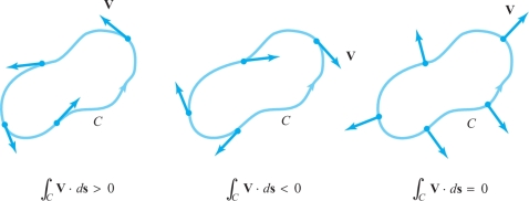
Let us pause to consider the physical meaning of \(\int_C {\bf V} \,{\cdot}\, d {\bf s}\) when \({\bf V}\) is the velocity field of a fluid. Suppose, for example, that \({\bf V}\) points in the direction tangent to the oriented curve \(C\) (Figure 18.16). Then clearly \(\int_C {\bf V} \,{\cdot}\, d {\bf s} > 0\), and particles on \(C\) tend to rotate counterclockwise. If \({\bf V}\) is pointing in the opposite direction, then \(\int_C {\bf V} \,{\cdot}\, d {\bf s} < 0\) and particles tend to rotate clockwise. If \({\bf V}\) is perpendicular to \(C\), then particles don't rotate on \(C\) at all and \(\int_C {\bf V} \,{\cdot}\, d {\bf s}=0\). In general, \(\int_C {\bf V} \,{\cdot}\, d {\bf s}\), being the integral of the tangential component of \({\bf V}\), represents the net amount of turning of the fluid in a counterclockwise direction around \(C\). We therefore refer to \(\int_C {\bf V} \,{\cdot}\, d {\bf s}\) as the circulation of \({\bf V}\) around \(C\) (see Figure 18.17).
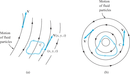
These results allow us to see just what curl \({\bf V}\) means for the motion of a fluid. The circulation \(\int_{\partial\! S_\rho} {\bf V} \,{\cdot}\, d {\bf s}\) is the net velocity of the fluid around \(\partial\! S_\rho\), so that (curl \({\bf V}) \,{\cdot}\, {\bf n}\) represents the turning or rotating effect of the fluid around the axis \({\bf n}\).
Circulation and Curl
The dot product of curl \({\bf V}({\rm P})\) with a unit vector \({\bf n}\), namely, curl \({\bf V}({\rm P})\, {\cdot} {\bf n}\), equals the circulation of \({\bf V}\) per unit area at P on a surface perpendicular to \({\bf n}\).
447
Observe that the magnitude of curl \({\bf V}{\rm (P)} \,{\cdot}\, {\bf n}\) is maximized when \({\bf n} = \hbox{curl } {\bf V} / \| \hbox{curl } {\bf V} \|\) (evaluated at P). Therefore, the rotating effect at P is greatest about the axis that is parallel to curl \({\bf V}/ \|\hbox{curl } {\bf V} \|\). Thus, curl \({\bf V}\) is aptly called the vorticity vector.
We can use these ideas to compute the curl in cylindrical coordinates.
example 4
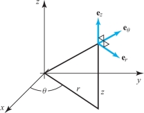
Let the unit vectors \({\bf e}_r,{\bf e}_\theta, {\bf e}_z\) associated with cylindrical coordinates be as shown in Figure 18.18. Let \({\bf F}=F_r {\bf e}_r+F_\theta{\bf e}_\theta +F_z{\bf e}_z\). (The subscripts here denote components of \({\bf F}\), not partial derivatives.) Find a formula for the \({\bf e}_r\) component of \({\nabla} \times {\bf F}\) in cylindrical coordinates.
solution Let \(S\) be the surface shown in Figure 18.19.
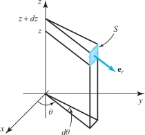
448
The area of \(S\) is \(r{\,d} \theta {\,d} z\) and the unit normal is \({\bf e}_r\). The integral of \(\bf F\) around the edges of \(S\) is approximately \begin{eqnarray*} && [F_\theta (r,\theta,z)-F_\theta (r,\theta,z+dz)]r{\,d} \theta+ [F_z(r,\theta+d \theta,z)-F_z(r,\theta,z)]{\,d} z\\[6pt] && \qquad\approx -\frac{\partial\! F_\theta}{\partial z}{\,d} z\, r{\,d} \theta + \frac{\partial\! F_z}{\partial \theta}\,d\theta\, d z. \end{eqnarray*}
Thus, the circulation per unit area is this expression divided by \(r {\,d} \theta\, d z\), namely, \[ \frac{1}{r}\frac{\partial\! F_z}{\partial \theta}-\frac{\partial\! F_\theta} {\partial z}. \]
According to the previous box, this must be the \({\bf e}_r\) component of the curl.
Gradient, Divergence, and Curl in Cylindrical and Spherical Coordinates
By similar arguments to Example 4, we find that the curl in cylindrical coordinates is given by \[ {\nabla} \times {\bf F}=\frac{1}{r} \left| \begin{array}{c@{\quad}c@{\quad}c} {\bf e}_r & r{\bf e}_{\theta} & {\bf e}_z\\[4pt] \displaystyle\frac{\partial\!}{\partial r} &\displaystyle\frac{\partial\!}{\partial \theta}&\displaystyle\frac{\partial\!}{\partial z}\\[8pt] F_r & {\it rF}_\theta & F_z \end{array} \right|. \]
We can find other important vector quantities expressed in different coordinate systems. For example, the chain rule shows that the gradient in cylindrical coordinates is \[ {\nabla}\! f=\frac{\partial\! f}{\partial r}\,{\bf e}_r +\frac{1}{r} \frac{\partial\! f}{\partial \theta}\,{\bf e}_\theta +\frac{\partial\! f}{\partial z}\,{\bf e}_z, \] and in Section 18.4 we will establish related techniques that give the following formula for the divergence in cylindrical coordinates: \[ {\nabla} \,{\cdot}\, {\bf F} =\frac{1}{r}\left[\frac{\partial\!}{\partial r}(r F_r)+ \frac{\partial\! F_\theta}{\partial \theta}+\frac{\partial\!}{\partial z}(r F_z)\right]. \]
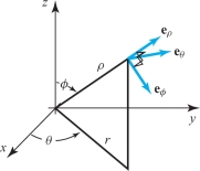
Corresponding formulas for gradient, divergence, and curl in spherical coordinates are \begin{eqnarray*} {\nabla}\! f &=& \frac{\partial\! f}{\partial\! \rho}\,{\bf e}_\rho+ \frac{1}{\rho} \frac{\partial\! f}{\partial \phi}\,{\bf e}_\phi +\frac{1}{\rho \sin \phi}\frac{\partial\! f}{\partial \theta}\,{\bf e}_\theta\\[6pt] {\nabla} \,{\cdot} \,{\bf F} &=& \frac{1}{\rho^2}\frac{\partial\!}{\partial\! \rho} (\rho^2 F_\rho)+\frac{1}{\rho \sin \phi}\frac{\partial\!}{\partial \phi}(\sin \phi F_\phi)+ \frac{1}{\rho \sin \phi}\frac{\partial\! F_\theta}{\partial \theta}\\[-15pt] \end{eqnarray*} and \begin{eqnarray*} {\nabla} \times {\bf F} &=&\left[ \frac{1}{\rho \sin \phi}\frac{\partial\!}{\partial \phi}(\sin \phi F_\theta)- \frac{1}{\rho \sin \phi}\frac{\partial\! F_\phi}{\partial \theta}\right]{\bf e}_\rho\\[6pt] && +\left[\frac{1}{\rho \sin \phi}\frac{\partial\! F_\rho}{\partial \theta}- \frac{1}{\rho}\frac{\partial\!}{\partial\! \rho}(\rho F_\theta)\right]{\bf e}_{\phi}+ \left[\frac{1}{\rho}\frac{\partial\!}{\partial\! \rho}(\rho F_\phi)-\frac{1}{\rho} \frac{\partial\! F_\rho}{\partial \phi}\right]{\bf e}_\theta, \end{eqnarray*} where \({\bf e}_\rho,{\bf e}_\phi,{\bf e}_\theta\) are as shown in Figure 18.20 and where \({\bf F}=F_\rho {\bf e}_\rho+F_\phi {\bf e}_\phi+F_\theta {\bf e}_\theta\).
Faraday’s Law
449
Vector calculus plays an essential role in the theory of electromagnetism. The next example shows how Stokes’ theorem applies.
example 5
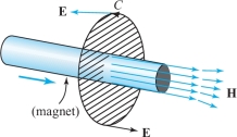
Let \({\bf E}\) and \({\bf H}\) be time-dependent electric and magnetic fields, respectively, in space. Let \(S\) be a surface with boundary \(C\). We define \begin{eqnarray*} \int_C {\bf E}\,{\cdot}\, d {\bf s} &=& \hbox{voltage around } C,\\[5pt] \intop\!\!\!\intop\nolimits_{S} {\bf H}\,{\cdot}\, d {\bf S} &=& \hbox{magnetic flux across } S.\\[-8pt] \end{eqnarray*}
Faraday’s law (see Figure 18.21) states that the voltage around C equals the negative rate of change of magnetic flux through S. Show that Faraday’s law follows from the following differential equation (one of the Maxwell equations): \[ {\nabla} \times {\bf E} =-\frac{\partial {\bf H}}{\partial t}. \]
solution Assume that \(-\partial {\bf H}/\partial t={\nabla} \times {\bf E}\) holds. By Stokes’ theorem, \[ \int_C {\bf E}\,{\cdot}\, d {\bf s}=\intop\!\!\!\intop\nolimits_{S} ({\nabla} \times {\bf E})\,{\cdot}\, d {\bf S}. \]
Assuming that we can move \(\partial\!/\partial t\) under the integral sign, we get \[ -\frac{\partial\!}{\partial t}\intop\!\!\!\intop\nolimits_{S}{\bf H}\,{\cdot}\, d {\bf S}=\intop\!\!\!\intop\nolimits_{S} - \frac{\partial {\bf H}}{\partial t}\,{\cdot}\, d {\bf S}=\intop\!\!\!\intop\nolimits_{S} (\nabla \times {\bf E})\,{\cdot}\, d {\bf S}=\int_C {\bf E}\,{\cdot}\, d {\bf s} \] and so \[ \int_C {\bf E}\,{\cdot}\, d {\bf s} =-\frac{\partial\!}{\partial t}\intop\!\!\!\intop\nolimits_{S} {\bf H}\,{\cdot}\, d {\bf S}, \] which is Faraday’s law.
Falling Cats and Stokes’ Theorem
Have you ever wondered how a falling cat can right itself? Released from a resting position with its feet above its head, the cat is able to execute a 180\(^{\circ}\) reorientation and land safely on its feet. This well-known phenomenon has fascinated people for many years—especially in cities like New York, where cats have been known to survive falls of 8 to 30 stories!
There have been many incorrect explanations as to how cats are able to right themselves, including the idea that it has to do with how the cat twirls its tail. This cannot be right because Manx cats, which have no tails, can also perform this feat!
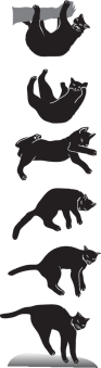
We observe, as in Figure 18.22, that the cat achieves this net change in orientation by wriggling, to create changes in its internal shape or configuration. On the surface, this provides a seeming contradiction; because the cat is dropped from a resting position, it has zero angular momentum at the beginning of the fall and hence, according to a basic law of physics called conservation of angular momentum, the cat has zero angular momentum throughout the duration of its fall.footnote # Amazingly, the cat has effectively changed its angular position while maintaining zero angular momentum!
450
The exact process by which this occurs is subtle; intuitive reasoning can lead one astray and, as we have indicated, many false explanations have been offered throughout the history of trying to solve this mystery.footnote # Recently, new and interesting insights have been discovered using geometric methods that, in fact, are related to curvature (see Section 7.7).footnote #
The way that curvature and geometry are related to the falling cat phenomenon is not easy to explain in full detail, but we can explain a similar phenomenon that is easy to understand. Interestingly, Stokes’ theorem is the key to understanding these types of phenomena.
For a discussion on how astronauts reorient themselves in space, click here.
Another example to help visualize this effect is to consider astronauts who wish to reorient themselves in a free-space environment. As with the falling cat, this motion can again be achieved using internal gyrations, or \({\it shape \ changes.}\) For instance, consider astronauts moving their arms much like the motion of arms stirring liquid in a large kettle. The arms are held out forward, to lie in a horizontal plane that goes through the shoulders, parallel to the floor; the hands are clasped together and remain in this horizontal plane during the circular stirring motion. At the point of maximum extension of the arms, the inertia of the body about a vertical axis is also at a maximum. Conservation of angular momentum requires that the body rotate in an opposite and proportional manner to the motion of the arms. As the arms rotate around and are brought in, however, the inertia of the body is reduced. The motion of the body in reaction is therefore also reduced. Thus, in one complete cycle of arm movement, the body undergoes a net rotation opposite the direction of arm motion. When the desired orientation is achieved, the astronaut needs merely to stop the arm motion in order to come to rest. One often refers to the extra motion that is achieved as \(\it geometric \ phase\).
Here is a link to a NASA video: "Zero-G: "Movement in Microgravity: Skylab to Space Shuttle" 1988 NASA Weightlessness Footage": https://www.youtube.com/watch?v=OvXKTOjaVQ4 that allows you to watch this in action. In particular, at 5:46 into the video, you can see astronauts reorienting their bodies in space without touching anything.
\({\bf Link \ with \ Non-Euclidean \ Geometry}\) The theory of geometric phases also shows up in an interesting way in non-Euclidean geometry---as in the geometry of triangles drawn on a sphere. A simple way to explain this link is as follows. Hold your hand at arm's length, but allow rotation in your shoulder joints. Move your hand along three great circles, forming a triangle on the sphere; during the motion along each arc, always keep your thumb \({\it parallel}\); that is, it should move in such a way that it forms a \({\it fixed}\) angle with the direction of motion along each arc and does not rotate when switching arcs. After completing the circuit around the triangle, your thumb will return rotated through an angle relative to its starting position (see Figure below). Can you see in the Figure that the angle of rotation is 90\(^\circ\) (or \(\pi\)/2 radians) and that this is what happens when you do the thumb experiment yourself?
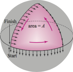
For general spherical triangles, this angle (in radians) is given by \(\Theta =\Delta -\pi\), where \(\Delta\) is the sum of the angles of the triangle. The fact that \(\Theta\) is strictly positive (!) is one of the basic truths of non-Euclidean geometry---the sum of the angles of a right triangle on a sphere is greater than \(\pi\)! This angle is also related to the \({\it area A}\) enclosed by the triangle through the relation \(\Theta =A/r^{2}\), where \(r\) is the radius of the sphere. The rotational shift of the thumb during the course of its cyclic journey around the spherical triangle is directly related to the curvature of the sphere and to the area enclosed by the path that is traced out. Notice first that for a spherical triangle that is \(1/8\) of the sphere, \(A = 4\pi r^{2} /8 = \pi r^{2}/2\). Thus, \(A/r^{2}=\pi /2\). Notice also that when \(r \to \infty \), the sphere becomes flatter and thus approaches a Euclidean plane, in which case \(\Theta = 0\).
The cyclic journey of the thumb around the closed path is analogous to the cyclic internal motions made by the cat during its fall; the 90\(^\circ\) shift in the direction of the thumb after one trip around is analogous to the 180\(^\circ\) reorientation of the cat. A deeper look at the underlying mathematics shows that, in fact, they are both instances of the same phenomenon (called \({\it holonomy}\) )---and Stokes' theorem is the key to understanding it.