Earth’s Magnetic Field and The Geodynamo

Like the mantle, Earth’s outer core transports most of its heat by convection. But the same techniques that have revealed so much about mantle convection—seismic tomography and the study of Earth’s gravitational field—have provided almost no information about convection in the core. Why not?

The problem has to do with the fluidity of the outer core. The mantle is a viscous solid that flows very slowly. As a result, convection creates regions where temperatures are significantly higher or lower than the average mantle geotherm. We can see these regions in Figure 14.11 as places where seismic wave velocities are lower or higher than the average at that depth. The outer core, in contrast, has a very low viscosity: its molten material can flow as easily as water or liquid mercury. Even small density variations caused by convection are quickly smoothed out by the rapid flow under the force of gravity. Any lateral variations in seismic wave velocity caused by convection will be much too small for us to see using seismic tomography, and they will not cause measurable distortions in the shape of the planet.

We can, however, investigate convection in the outer core through observations of Earth’s magnetic field. In Chapter 1, we briefly described the magnetic field and its generation by the geodynamo in the outer core. In Chapter 2, we discussed magnetic reversals and the use of magnetic anomalies in volcanic rocks to measure seafloor spreading. In this section, we will further explore the nature of Earth’s magnetic field and its origin in the geodynamo.

The Dipole Field

The most basic instrument used for sensing Earth’s magnetic field is the magnetic compass, invented by the Chinese more than 22 centuries ago. For hundreds of years, explorers and ship captains used magnetic compasses to navigate, but they had little understanding of how these ancient devices actually worked. In 1600, William Gilbert, physician to Queen Elizabeth I, provided a scientific explanation. He proposed that “the whole Earth is itself a great magnet” whose field acts on the small magnet of a compass needle to align it in the direction of the north magnetic pole.

Scientists of Gilbert’s day had begun to visualize a magnetic field as lines of force, such as those revealed by the alignment of iron filings on a piece of paper above a bar magnet. Gilbert showed that Earth’s magnetic lines of force point into the ground at the north magnetic pole and outward at the south magnetic pole, as if a powerful bar magnet were located at Earth’s center and oriented along an axis inclined about 11° from Earth’s axis of rotation (see Figure 1.17). In other words, the lines of force revealed a dipole (two-pole) magnetic field.

Complexity of the Magnetic Field

Gilbert solved an important problem for a seafaring nation dependent on the compass for navigation, but his explanation was only partly correct. We now know that the source of the magnetic field is a geodynamo powered by core convection, not a permanent magnet at Earth’s center (which would be quickly destroyed by the high temperatures in the core). The geodynamo is formed by rapid convective movements in the liquid, iron-rich, electrically conducting outer core. The magnetic field produced by the geodynamo is considerably more complex than a simple dipole field, and it is constantly changing over time due to these fluid movements.

Earth Issues: 14.2 The Geoid: The Shape of Planet Earth

The surface of the ocean is warped upward in places where the pull of Earth’s gravitational field is stronger and downward where the pull is weaker. The shape of the ocean’s surface can be precisely measured by radar altimeters mounted on satellites. By averaging out wave motions and other fluctuations, oceanographers can map the small-scale variations in gravity caused by geologic features on the seafloor, such as faults and seamounts (see Chapter 20). Variations in gravity are also produced by the much larger features caused by mantle convection currents.

A perfectly still ocean would have a surface that conforms to what geologists call the geoid. The surface of a still body of water is perfectly “flat” in the sense that the pull of gravity is perpendicular to that surface—otherwise, the water would flow “downhill” to make the surface flatter. The geoid is defined as an imaginary surface at some reference height above Earth adjusted to be everywhere perpendicular to the local gravitational force. Because the ocean surface approximates the geoid, we usually take the reference height to be sea level. When we measure the height of a mountain relative to sea level, we are actually measuring its height above the geoid at that point. In this sense, the geoid is simply the shape of Earth. Geologists can use the geoid to calculate the strength and direction of the gravitational force at any point on the planet’s surface and infer how rock density varies in Earth’s interior.

Radar altimeters can easily map the geoid over the oceans, but how can we get this information on dry land? It turns out that the geoid can be measured for the entire Earth by tracking orbiting satellites. Three-dimensional mass variations in the mantle exert a small gravitational pull on the satellites, shifting their orbits slightly. By monitoring these shifts over long periods, scientists can create a two-dimensional map of the geoid over continents as well as oceans.

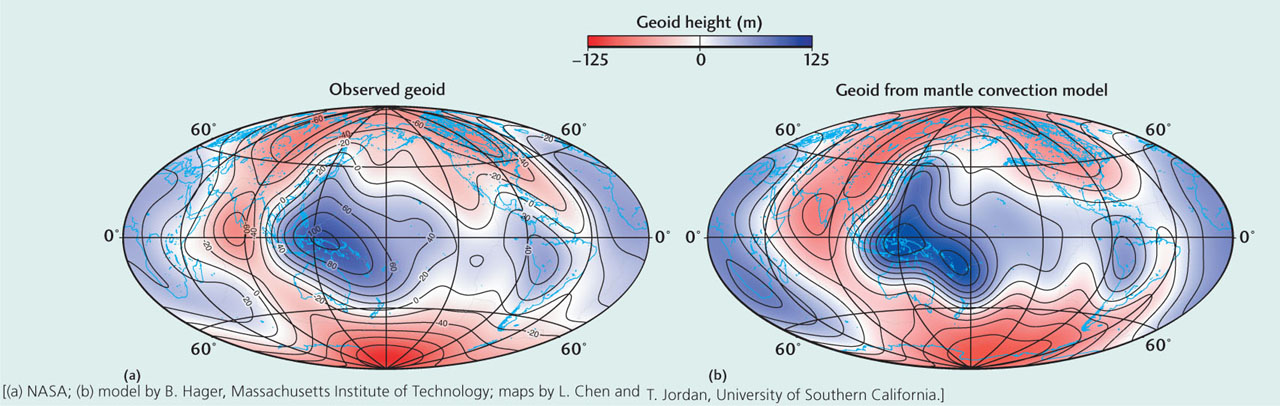
A smoothed version of the observed geoid reveals the large-scale features of Earth’s gravitational field. Relative to what sea level would be on an Earth without any lateral variation in mass, the elevation of the geoid varies from a low of about 2110 m at a point near the coast of Antarctica to a high of just over 100 m on the island of New Guinea in the western Pacific.

The geoid shows some similarities to the large-scale features of the deeper parts of the mantle, as you can see by comparing the geoid map with Figures 14.11d and e. This agreement suggests that the three-dimensional variations in both rock density and S-wave velocity are related to temperature differences arising from mantle convection.

Geophysicists Brad Hager and Mark Richards tested this hypothesis in the mid-1980s. Using laboratory data for calibration, they first calculated three-dimensional density variations from the seismic wave velocity variations mapped by seismic tomography. They then constructed a computer model of convective flow by assuming that the heavier parts of the mantle are sinking while the lighter parts are rising. Finally, they calculated what the geoid shape should be according to this convection model. You can see that their model results match the observed geoid quite well, especially for the largest features. This agreement has given geologists confidence that temperature variations within the mantle convection system can explain what we see both in seismic images and in the gravitational field.

A smoothed map of the geoid, or “shape of Earth,” derived from satellite observations. The contours, given here in meters, show how the observed sea level deviates from that on an ideal Earth without any lateral variation in rock density. (b) A map of the geoid computed from a model of mantle convection that is consistent with the temperature structure of the mantle derived from seismic tomography. By matching the observed geoid with such theoretical models, geologists have improved their understanding of the mantle convection system.

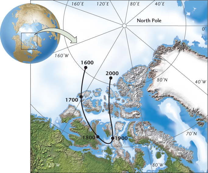
Within a few decades after Gilbert’s famous pronouncement, careful observers had realized that the magnetic field varies over time. Not surprisingly, some of the best evidence for these changes came from the compass measurements systematically recorded by the British navy. Navigators had to correct their compass bearings to account for the displacement of the north magnetic pole (magnetic north) from the north rotational pole (true north), and these corrections showed that the north magnetic pole was moving at rates of 5° to 10° per century (Figure 14.12). Little did the British sailors know that these changes were caused by convective movements deep in Earth’s core!

Figure 14.12: Path of the north magnetic pole, as mapped by compass readings and other measurements of Earth’s magnetic field since 1600. Changes in the pole location are caused by convective movements within Earth´s fluid outer core.

The Nondipole Field

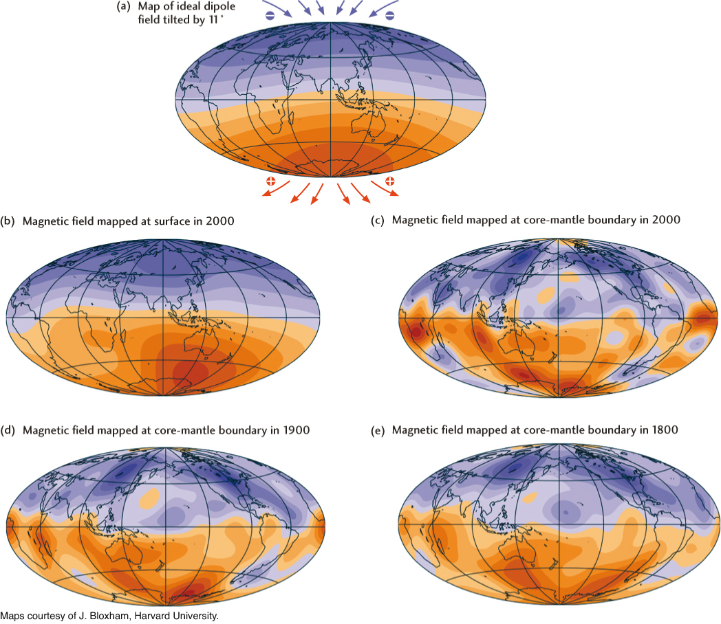
Measurements at Earth’s surface have revealed that only about 90 percent of Earth’s magnetic field can be described by the simple dipole field illustrated in Figure 1.17. The remaining 10 percent, which geologists refer to as the nondipole field, has a more complex structure. This structure can be seen by comparing the magnetic field strengths calculated for a simple dipole field (Figure 14.13a) with those of the observed field (Figure 14.13b). If we extrapolate the observed lines of force down to the core-mantle boundary using a computer model, the size of the nondipole field actually increases relative to the size of the dipole field, as indicated by the bumpiness of the orange and blue colors on the map in Figure 14.13c. The poorly conducting mantle tends to smooth out complexities in the magnetic field, making the dipole field seem bigger than it really is.

Figure 14.13: Earth’s magnetic field changes over time. Blue colors show the strength of the inward-pointing field, and orange colors show the strength of the outward-pointing field. The magnetic field mapped at the surface (b) is more complex than a simple dipole (a), and it shows more complications when extrapolated to the core-mantle boundary (c). The features on the nondipole field change over time, as seen in (c) through (e), owing to convection in Earth’s fluid outer core.

Secular Variation

Magnetic records for the last 300 years (many from the British navy) show that both the dipole and nondipole components of Earth’s magnetic field are changing over time, but that this secular (time-related) variation is fastest for the nondipole component. Secular variation is evident when we compare a map of today’s magnetic field at the core-mantle boundary (Figure 14.13c) with maps reconstructed for previous centuries (Figure 14.13d, e). Changes in field strength occur on time scales of decades and indicate that fluid movements within the geodynamo are on the order of millimeters per second.

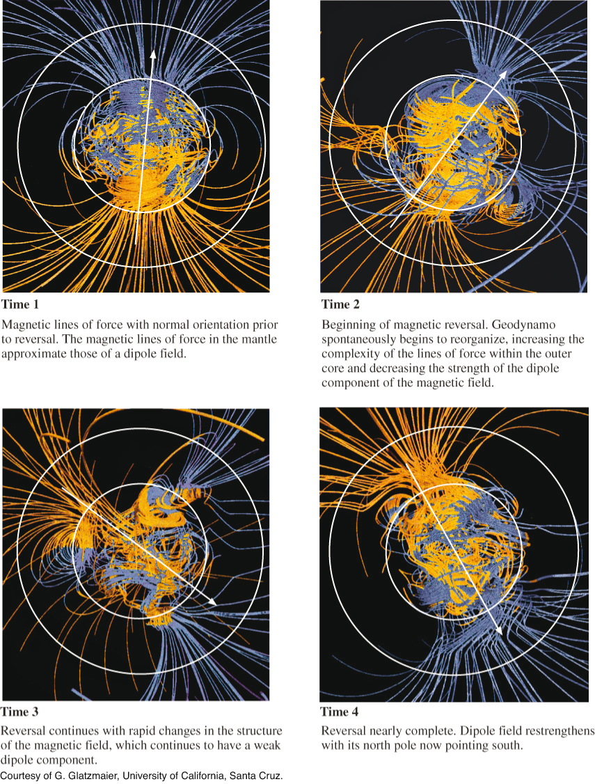
Scientists can use this secular variation to help them understand convection in the outer core. With high--performance computers, they have been able to simulate the complex convective movements and electromagnetic interactions in the outer core that might be creating the geodynamo. The magnetic lines of force from one such simulation are shown in Figure 14.14. Away from the core, the lines of force can be approximated by a dipole field, but they become more complicated near the core-mantle boundary. Within the core itself, they are hopelessly entangled by the strong convective movements.

Figure 14.14: Computer models have shown that spontaneous changes in the geodynamo could cause magnetic reversals.

Magnetic Reversals

These same computer simulations also allow us to understand a remarkable behavior of the geodynamo: spontaneous reversals of the magnetic field. As discussed in Chapter 2, the magnetic field reverses its direction at irregular intervals (ranging from tens of thousands to millions of years), exchanging the north and south magnetic poles as if the magnet depicted in Figure 1.16 were flipped 180°. Recent computer simulations of the geodynamo were able to reproduce these sporadic reversals in the absence of any external triggers (Figure 14.14). In other words, it is possible for Earth’s magnetic field to reverse itself spontaneously, purely through internal interactions.

This behavior illustrates a fundamental difference between the geodynamo and the dynamos used in power plants. A steam-powered dynamo is an artificial system engineered by humans to do a particular job. The geodynamo, in contrast, exemplifies a self-organized natural system—one whose behavior is not predetermined by external constraints, but emerges from interactions within the system. The other two global geosystems, the plate tectonic and climate systems, also display a wide variety of self-organized behaviors. Understanding how these natural systems organize themselves is one of the greatest challenges to geoscience. We will return to this subject when we discuss the climate system in Chapter 15.

Paleomagnetism

We have seen repeatedly how the geologic record of ancient magnetism, or paleomagnetism, has provided crucial information for understanding Earth’s history. Magnetic anomalies mapped on oceanic crust confirmed the existence of seafloor spreading, and they still provide the best data for tracking plate movements since the breakup of Pangaea 200 million years ago (see Chapter 2). Paleomagnetic data from old continental rocks have been essential for establishing the existence of earlier supercontinents, such as Rodinia (see Chapter 10).

Scientists have also used paleomagnetic data to reconstruct the history of Earth’s magnetic field. The oldest magnetized rocks found so far, which formed about 3.5 billion years ago, indicate that Earth had a magnetic field similar to the present one at that time. The presence of magnetization in the most ancient rocks is consistent with the ideas about Earth’s differentiation discussed in Chapter 1, which imply that a convecting liquid core must have been established very early in Earth’s 4.5-billion-year history.

Let’s delve a little more deeply into the rock-forming processes that have allowed geologists to draw these remarkable conclusions. You may find it helpful to consult the material in Figure 2.12 and its accompanying text as you read this section.

Thermoremanent Magnetization

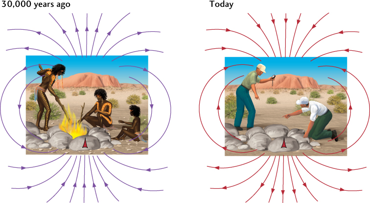
In the early 1960s, an Australian graduate student found a fireplace in an ancient campsite where Aborigines had cooked their meals. He carefully removed several stones that had been baked by the fires, first noting their physical orientation. Then he measured the direction of the stones’ magnetization and found that it was exactly the reverse of Earth’s present magnetic field. He proposed to his disbelieving professor that, as recently as 30,000 years ago, when the campsite was occupied, the direction of the magnetic field was the reverse of the present one—that is, a compass needle would have pointed south rather than north.

Recall that high temperatures destroy magnetization. An important property of many magnetizable materials is that, as they cool below about 5008C, they become magnetized in the direction of the surrounding magnetic field. This happens because groups of atoms of the material align themselves in the direction of the magnetic field when the material is hot. When the material has cooled, these atoms are locked in place. This process is called thermoremanent magnetization, because the magnetization caused by heating and cooling is “remembered” by the rock long after the magnetizing field has disappeared. Thus, the Australian student was able to determine the direction of Earth’s magnetic field at the time the stones cooled after the last campfire (Figure 14.15).

Figure 14.15: The orientation of Earth’s magnetic field 30,000 years ago was the reverse of today’s, as evidenced by magnetized rocks found in the fireplace of an ancient campsite. The rocks, when cooling after the last fire, became magnetized in the direction of the ancient magnetic field, leaving a permanent record of its orientation.

Thermoremanent magnetization is the same process that magnetizes lava flows and newly formed oceanic crust, as described in Chapter 2. The discovery of magnetic reversals in these igneous rock types was a key ingredient in formulating the theory of plate tectonics.

Depositional Remanent Magnetization

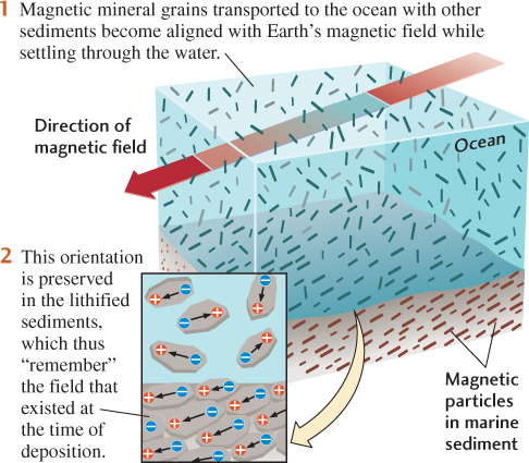
Some sedimentary rocks can take on a different type of remanent magnetization. Marine sedimentary rocks form when particles of sediment that have settled to the seafloor become lithified. Magnetic grains among the particles—chips of the mineral magnetite (Fe₃O₄), for example—become aligned in the direction of Earth’s magnetic field as they fall through the water, and this orientation may be incorporated into the rock when the sediments become lithified. The depositional remanent magnetization found in some sedimentary rocks results from the parallel alignment of all these tiny magnets, as if they were compasses pointing in the direction of the magnetic field prevailing at the time of deposition (Figure 14.16).

Figure 14.16: Newly formed sediments can become magnetized in the direction of the magnetic field at the time of their deposition.

Paleomagnetic Stratigraphy

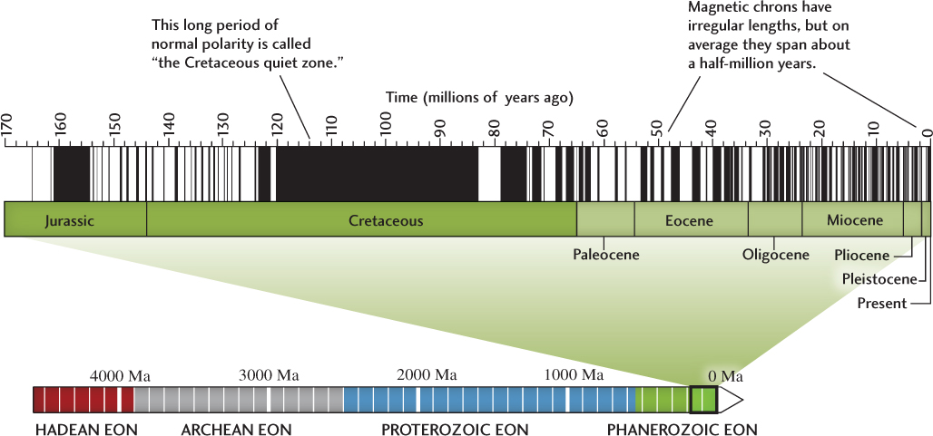
Geologists have used paleomagnetism in combination with isotopic dating methods to work out the time sequence of magnetic reversals over the last 170 million years (Figure 14.17). This information can be used, in turn, to date new rock formations. Paleomagnetic stratigraphy is useful to archaeologists and anthropologists as well as to geologists. For example, the paleomagnetic stratigraphy of continental sediments has been used to date sediments containing the remains of predecessors of our own species.

Figure 14.17: The paleomagnetic time scale from 170 million years ago to the present, showing normal chrons (black bands) and reversed chrons (white bands).

As we saw in Chapter 2, periods of “normal” (same as today) and reversed magnetic field orientation, which are called magnetic chrons, have irregular lengths, but on average they last about a half-million years. Superimposed on the chrons are transient, short-lived reversals known as subchrons, which may last anywhere from several thousand years to tens of millions of years. The reversal found in the rocks remagnetized by the Australian Aborigines’ campfire (see Figure 14.15) can be interpreted as a reversed subchron within the present normal magnetic chron.

The Magnetic Field and the Biosphere

From the rock record, we know that the geodynamo began to operate early in Earth’s history, and that life therefore evolved within a strong magnetic field. The consequences turn out to be rather surprising. For example, many types of organisms—pigeons, sea turtles, whales, and even bacteria—have evolved sensory systems that use the magnetic field for navigation (Figure 14.18). Their basic sensors are small crystals of magnetite that become magnetized by Earth’s magnetic field as they are biologically precipitated within the organism (see Figure 11.8b). These crystals act as tiny compasses to orient the organism within the magnetic field. Geobiologists have discovered that some animals can even use arrays of magnetite crystals to sense the strength of the magnetic field, which provides them with additional information for navigation.

Figure 14.18: A flock of homing pigeons preparing to land at their coop in Cuba’s Villaclara province after a 240-km flight across the island from Havana. These birds use Earth’s magnetic field to navigate the long flights back to their homes. Recent evidence suggests that homing pigeons sense the magnetic field using receptors in their inner ears and beaks.

The magnetic field is not just a convenient frame of reference for flying and swimming species. It constitutes a part of the Earth system that is essential for sustaining a rich and delicate biosphere at the planet’s surface. Although the machinery of the geodynamo operates deep within the core, its magnetic lines of force reach far into outer space, forming a barrier that shields Earth’s surface from the damaging radiation of the solar wind (see Figure 1.18). Without the protection of a strong magnetic field, this intense stream of high-energy, electrically charged particles would be lethal to many organisms.

Moreover, if the geodynamo were to stop producing a magnetic field, bombardment by the solar wind would gradually strip away Earth’s atmosphere, further degrading the terrestrial environment. This appears to have happened in the case of Mars. Paleomagnetism in the ancient Martian crust has been detected by orbiting spacecraft, so we know the Red Planet once had an active geodynamo that generated a strong magnetic field. Sometime early in the planet’s history, however, its geodynamo ceased to operate, perhaps because the Martian core cooled enough to freeze. Exposure to the solar wind subsequently eroded its atmosphere to the tenuous state we observe today.