Climate Variation

Earth’s climate varies considerably from place to place: its poles are frigid and arid, its tropics sweltering and humid. Comparable variations in climate can also occur over time. The geologic record shows us that periods of global warmth have alternated with periods of glacial cold many times in the past. This climate variation is erratic; dramatic changes can happen in just a few decades or evolve over time scales of many millions of years.

Some climate variation can be attributed to factors outside the climate system, such as solar forcing and changes in the distribution of land and sea surfaces caused by continental drift. Others result from changes within the climate system itself, such as the growth of continental glaciers that increase Earth’s albedo. Both types of variations, external and internal, can be amplified or suppressed by feedbacks. In this section, we will examine several types of climate variation and discuss their causes, beginning with short-term variation on a regional scale.

Short-Term Regional Variations

Local and regional climates are much more variable than the average global climate: averaging over large surface areas, like averaging over time, tends to smooth out small-scale fluctuations. Over periods of years to decades, the predominant regional variations result from interactions between atmospheric circulation and sea and land surfaces. They generally occur in distinct geographic patterns, although their timing and amplitudes can be highly irregular.

One of the best-known examples is a warming of the eastern Pacific Ocean that occurs every 3 to 7 years and lasts for a year or so. Peruvian fishermen call such an event El Niño (“the boy child” in Spanish) because the warming typically reaches the surface waters off the coast of South America around Christmastime. El Niño events can decimate fish populations, which depend on the upwelling of cold water for their nutrient supply, and can thus be disastrous for coastal human populations that depend on fishing.

Scientists have shown that El Niño and a complementary cooling event, known as La Niña (“the girl child”), are part of a natural variation in the exchange of heat between the atmosphere and the tropical Pacific Ocean. This variation is known as the El Niño–Southern Oscillation, or ENSO (Figure 15.9).

Figure 15.9: The El Niño–Southern Oscillation (ENSO) is a natural variation in the exchange of heat between the atmosphere and the surface waters of the tropical Pacific Ocean.

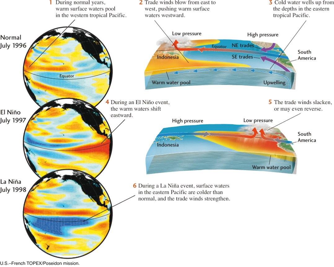
Normally, atmospheric pressure gradients cause prevailing winds, the trade winds, to blow from east to west, pushing the warm tropical waters westward. This movement of water causes colder water to well up from the ocean depths off Peru. Sporadically, the trade winds weaken or occasionally even reverse direction, cutting off the upwelling and equalizing water temperatures across the tropical Pacific (an El Niño event). At other times, the trade winds strengthen, enhancing the temperature difference between the eastern and western Pacific (a La Niña event). This recurring swing in air pressure is called the Southern Oscillation.

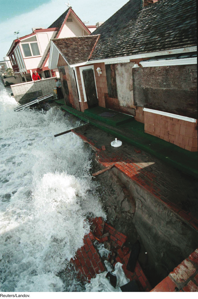
In addition to disrupting the eastern Pacific fishery, El Nino has been implicated in triggering changes in wind and rain patterns over much of the globe. The 1997–1998 El Niño was the strongest on record, and it contributed to droughts in Australia and Indonesia; heavy rains and flash floods in Peru, Ecuador, and Kenya; and storms in California that caused landslides and floods (Figure 15.10). Crops failed and fisheries were decimated in many areas. According to one estimate, the global disruption in weather patterns and ecosystems may have cost 23,000 lives and caused $33 billion in damage.

Figure 15.10: Storm waves associated with the 1997–1998 El Niño attacking homes along the Pacific coastline in Del Mar, California.

Climate scientists have identified similar patterns of weather and climate variation in other regions. One example is the North Atlantic Oscillation, a highly irregular fluctuation in the balance of atmospheric pressures between Iceland and the Azores that has a strong influence on the movement of storms across the North Atlantic and thus affects weather conditions throughout Europe and parts of Asia. A better understanding of these patterns is improving long-range weather forecasting and may provide important information about the regional effects of human-induced climate change.

Long-Term Global Variations: The Pleistocene Ice Ages

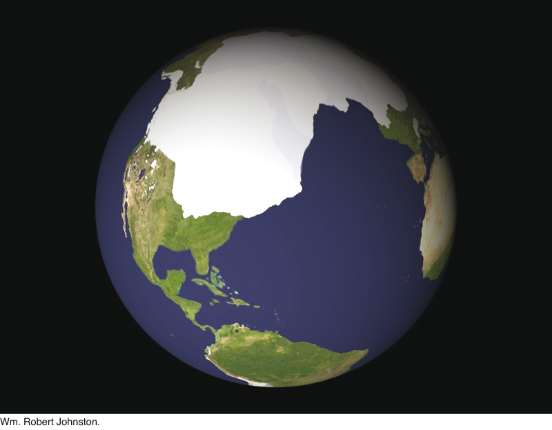
Some of the most dramatic climate variations that can be seen in the geologic record are the glacial cycles of the Pleistocene epoch, which began 1.8 million years ago. A glacial cycle begins with a gradual decline in temperature of about 6°C to 8°C from a warm interglacial period to a cold glacial period, or ice age. As the climate cools, water is transferred from the hydrosphere to the cryosphere. The amount of sea ice increases, and more snow falls on the continents in winter than melts in summer, increasing the volume and area of polar ice caps and decreasing the volume of the oceans. As the ice caps expand into lower latitudes, they reflect more solar energy back into space, and Earth’s surface temperatures fall further—an example of albedo feedback. Sea level falls, exposing areas of the continental shelves that are normally under water. At the peak of the ice age—the glacial maximum—great continental glaciers up to 2 or 3 m thick cover vast land areas (Figure 15.11). The ice age ends abruptly with a rapid rise in temperature. Water is transferred from the cryosphere to the hydrosphere as the ice caps melt and sea level rises.

Figure 15.11: At the last glacial maximum around 20,000 years ago, continental glaciers covered most of North America. The continental shelves were exposed by the lowering of the sea level, illustrated here by the expanded coastline of Florida.

Timing the Pleistocene Ice Ages

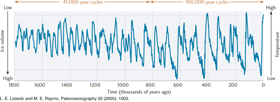
A precise record of Pleistocene temperature variations can be obtained by measuring oxygen isotopes preserved in marine sediments and in glacial ice. Pleistocene marine sediments contain numerous fossils of foraminifera: small, single-celled marine organisms that secrete shells of calcite (CaCO₃). The proportions of oxygen isotopes incorporated into these shells depend on the oxygen isotope ratio of the seawater in which the organisms lived. Water (H₂O) containing the lighter and more common isotope, oxygen-16 (¹⁶O), has a greater tendency to evaporate than water containing the heavier oxygen-18 (¹⁸O). Therefore, during ice ages, ¹⁸O is preferentially left behind in the oceans as water containing ¹⁶O evaporates from the ocean surface and is trapped in glacial ice, and the ¹⁸O/¹⁶O ratio in the oceans rises. Paleoclimatologists can use ¹⁸O/¹⁶O ratios in marine sediment beds to estimate sea surface temperature and ice volume at the time the beds were deposited. Figure 15.12 shows changes in global climate over the last 1.8 million years as inferred from these estimates.

Figure 15.12: Changes in global climate over the last 1.8 million years, as inferred from oxygen isotope ratios in marine sediments. The peaks indicate interglacial periods (high temperatures, low ice volumes, high sea level), and the valleys indicate ice ages (low temperatures, high ice volumes, low sea level).

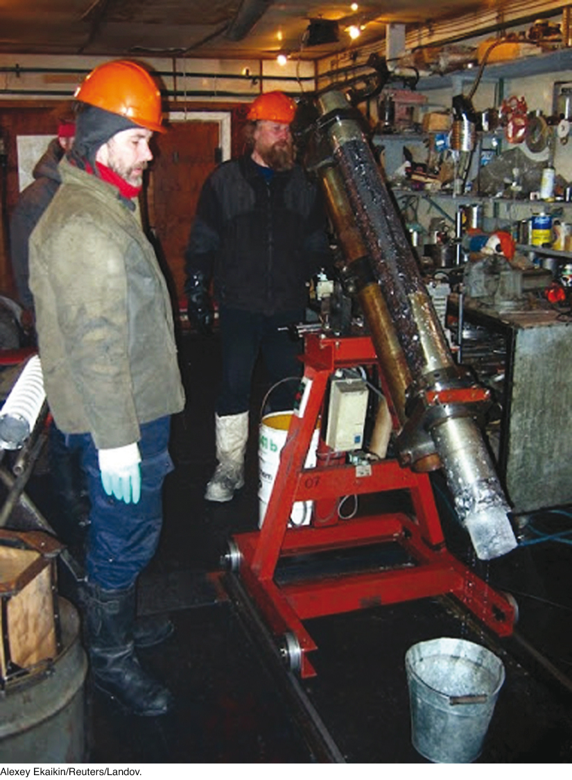
Earth Issues: 15.1 Ice-Core Drilling in Antarctica and Greenland

At the Vostok Station in the frozen Antarctic, Russian and French scientists have worked for decades to uncover the climatological history of Earth hidden in glacial ice. In the 1970s and 1980s, they drilled boreholes 2000 m deep into the East Antarctic ice sheet and brought up a set of ice cores for detailed laboratory study. The cores contained layers of ice produced by annual cycles of ice formation from snow. By carefully counting the layers, working from the top down, the researchers were able to infer the age of the ice with depth, much as tree rings are used to reveal the age of a tree. They measured oxygen isotope ratios in the ice as well as the gas composition of small bubbles trapped in the ice. From this stratigraphic record, they produced a detailed history of glacial cycles over the last 160,000 years.

By 1998, the ice borers at Vostok had drilled to a depth of 3600 m, penetrating ice accumulated over the past four glacial cycles and extending the climate record to more than 400,000 years ago. The data supported other evidence suggesting that variations in Earth’s orbit—Milankovitch cycles—control the alternation of ice ages and interglacial periods, and they showed that surface temperatures were correlated with concentrations of greenhouse gases in the atmosphere (see Figure 15.12). The Vostok results have been confirmed by ice core drilling at a number of other locations on the Antarctic and Greenland ice sheets.

These triumphs have not been won easily. The Vostok Station, located at an elevation of 3500 m near the center of Antarctica (its location is marked on the map of Figure 21.6), is an especially grueling place to do research. Its average annual temperature is only −55°C, and the lowest reliably measured temperature on Earth’s surface, −89.2°C, was recorded there in 1983. The scientists not only had to endure these extreme conditions, but also had to be careful not to melt and contaminate the ice cores while drilling them, transporting them to laboratories, and storing them. And they had to guard against misleading results—caused, for example, by the reaction of CO₂ with impurities in the ice. It is a tribute to the patience and ingenuity of these hardy bands of researchers that glacial ice cores have contributed so much to our understanding of the history of global climate change.

Russian scientists at the Vostok Station carefully remove an ice core from a drill. The layers produced by annual cycles of ice formation are visible in the core.

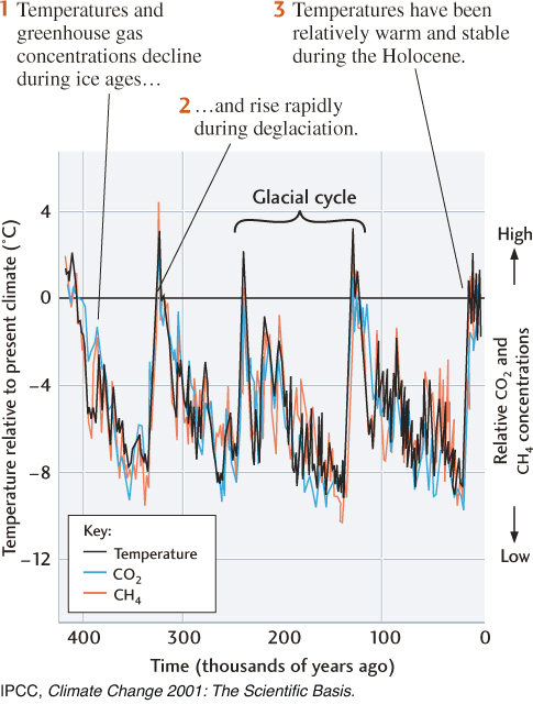
As ¹⁸O/¹⁶O ratios in the oceans increase during ice ages, those in the layers of ice that form the growing glaciers decrease. The best records of climate variation during the last half-million years come from ice cores drilled in the East Antarctic ice sheet by Russian scientists at the Vostok Station and in the Greenland ice sheet by European and U.S. teams (see Earth Issues 15.1). The oxygen isotope ratios of the ice layers in the cores can be used to estimate atmospheric temperatures at the time the ice formed. The composition of the atmosphere, including the concentrations of carbon dioxide and methane, can also be measured in tiny bubbles of air trapped at the time the ice formed. Figure 15.13 displays these three types of measurements from the Vostok ice core.

Figure 15.13: Three types of data were recovered from the Vostok Station ice cores, which were drilled to a depth of 3600 m in the East Antarctic ice sheet. Temperatures were estimated from oxygen isotope ratios. Carbon dioxide and methane concentrations came from measurements of air samples trapped as tiny bubbles within the Antarctic ice.

Milankovitch Cycles

The major ups and downs in the marine sediment record (see Figure 15.12) during the Pleistocene epoch match the glacial cycles in the ice core record (see Figure 15.13). Why does the climate fluctuate in such a pattern? Solar forcing is an obvious possibility. We know that it gets cold in winter because the amount of sunlight that falls at a particular latitude decreases due to the tilt of Earth’s axis. Could periods of glacial cold be explained by decreases in solar energy input over much longer time scales?

The answer appears to be yes. There are indeed small periodic variations in the amount of radiation Earth receives from the Sun. These variations are caused by Milankovitch cycles, periodic variations in Earth’s movement around the Sun, named after the Serbian geophysicist who first calculated them in the early twentieth century. Three kinds of Milankovitch cycles can be correlated with global climate variation (Figure 15.14).

Figure 15.14: Three kinds of Milankovitch cycles (much exaggerated in these diagrams) affect the amount of solar radiation Earth receives. (a) Eccentricity is the degree of ellipticity of Earth’s orbit. (b) Tilt is the angle between Earth’s axis of rotation and the angle perpendicular to the orbital plane. (c) Precession is the wobble of the axis of rotation. One can imagine this motion by thinking of the wobble of a spinning top.

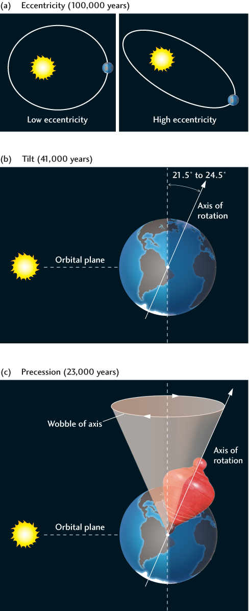
First, the shape of Earth’s orbit around the Sun changes periodically, becoming more circular at some times and more elliptical at others. The degree of ellipticity of Earth’s orbit around the Sun is known as its eccentricity. A nearly circular orbit has low eccentricity, and a more elliptical orbit has high eccentricity (Figure 15.14a). The amount of solar radiation Earth receives, averaged over its surface, varies slightly with eccentricity. The length of one cycle of variation in eccentricity is about 100,000 years.

Second, the angle or tilt of Earth’s axis of rotation changes periodically. Today this angle is 23.58, but it cycles between 21.58 and 24.58 with a period of about 41,000 years. These variations also slightly change the amount of radiation Earth receives from the Sun (Figure 15.14b).

Third, Earth’s axis of rotation wobbles like a top, giving rise to a pattern of variation called precession with a period of about 23,000 years (Figure 15.14c). Precession, too, modifies the amount of radiation Earth receives from the Sun, though by less than variations in eccentricity and tilt.

Correlations between Milankovitch Cycles and Glacial Cycles

You can see lots of small ups and downs in the record in Figure 15.12, but in the last half-million years, the record reveals a sawtooth pattern of major glacial cycles that looks roughly like this:

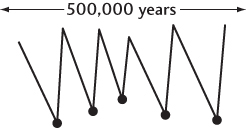
In particular, you can count five glacial maxima, in which ice volumes are high and temperatures are low (shown in the sketch above as black dots), revealing an average time interval between glacial maxima of about 100,000 years. This 100,000-year spacing of minimum temperatures closely matches the times of high orbital eccentricity, when Earth received slightly less radiation from the Sun—a Milankovitch cycle.

Now let’s move backward in time to examine the first half-million years of the record, in Figure 15.12, from 1.8 million to 1.3 million years ago. Again, we see many small fluctuations, but major maxima and minima occur more frequently than they do in the later record, as approximated in the following sketch:

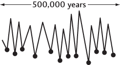
During this period, we find 12 glacial maxima, with an average spacing between them of about 41,000 years (500,000 years/12 cycles = 41,667 years per cycle). This shorter interval is very close to the 41,000-year cycle of variation in the tilt of Earth’s axis—another Milankovitch cycle! Like the variation in eccentricity, the variation in tilt is very small—only about 3° (see Figure 15.14b)—but it’s evidently enough to trigger ice ages.

The small changes in solar radiation caused by Milankovitch cycles cannot by themselves explain the large drops in Earth’s surface temperature from interglacial periods to ice ages. Some type of positive feedback must be operating within the climate system to amplify the solar forcing. The data in Figure 15.13 strongly suggest that this feedback involves greenhouse gases. Atmospheric concentrations of carbon dioxide and methane precisely track the temperature variations throughout the glacial cycles: warm interglacial periods are marked by high concentrations, cold glacial periods by low concentrations. Exactly how this feedback works has not yet been fully explained, but it demonstrates the importance of the greenhouse effect in long-term climate variations.

Many other aspects of this story are not yet understood. For example, you will notice in Figure 15.12 that the 41,000-year periodicity continued to dominate the climate record up to about 1 million years ago. Then, the highs and lows became more variable, eventually shifting to the 100,000-year periodicity after about 700,000 years ago. What caused this transition? Climate scientists are still scratching their heads.

In fact, we don’t really know what triggered the Pleistocene ice ages. The climate record shows that the 41,000-year glacial cycles were not confined to the Pleistocene, but extended back at least into the Pliocene epoch (5.3 million to 1.8 million years ago), when Antarctica became covered in ice. The global cooling of Earth’s climate that preceded these glaciations began during the Miocene epoch (23 million to 5.3 million years ago). Its cause continues to be debated, although most geologists believe it is somehow related to continental drift. According to one hypothesis, the collision of the Indian subcontinent with Eurasia and the resulting Himalayan orogeny led to an increase in the weathering of silicate rocks, and the chemical reactions of weathering decreased the amount of CO₂ in the atmosphere. Other hypotheses are based on changes in oceanic circulation associated with the opening of the Drake Passage between South America and Antarctica (25 million to 20 million years ago) or the closing of the Isthmus of Panama between North and South America (about 5 million years ago). Perhaps the cooling resulted from a combination of these events.

Long-Term Global Variations: Paleozoic and Proterozoic Ice Ages

In addition to the Pleistocene ice ages, there is good evidence in the geologic record for earlier episodes of continental glaciation during the Permian-Carboniferous and Ordovician periods and at least twice in the Proterozoic eon. In most cases, these events can be explained by plate tectonic processes, coupled with albedo feedback and other feedbacks in the climate system.

For most of Earth’s history, there were no extensive land areas in the polar regions, and there were no ice caps. Oceanic circulation extended from equatorial regions into polar regions, transporting heat and helping the atmosphere to distribute temperatures fairly evenly over Earth’s surface. When large land areas drifted to positions that obstructed this efficient transport of heat, the differences in temperature between the poles and the equator increased. As the poles cooled, ice caps formed. Some geologists believe that at one time in the late Proterozoic, Earth was completely covered by ice, and that only greenhouse gases emitted into the atmosphere by volcanoes allowed it to warm up again. We’ll take a closer look at this “Snowball Earth hypothesis” in Chapter 21.

Variations During the Most Recent Glacial Cycle

Within glacial cycles, temperatures do not vary smoothly over time (see Figure 15.13). Superimposed on the 100,000-year glacial cycles are climate fluctuations of shorter duration, some nearly as large as the changes from glacial to interglacial periods. Geologists have combined information from cores in continental and valley glaciers, lake- sediments, and deep-sea sediments to reconstruct a decade-by-decade—and in some cases, a year-by-year—history of short-term climate variations during the most recent glacial cycle.

The most recent ice age is known as the Wisconsin glaciation. Temperatures began to drop about 120,000 years ago, but reached their lowest values only about 21,000 to 18,000 years ago (the Wisconsin glacial maximum). Temperatures then rebounded to warm interglacial levels 11,700 years ago, marking the end of the Pleistocene and the beginning of the Holocene. Here we summarize some of the basic features of this remarkable chronicle.

• During the Wisconsin glaciation, Earth’s climate was highly variable, with shorter (1000-year) temperature oscillations occurring within longer (10,000-year) cycles. The most extreme variations appear to have been in the North Atlantic region, where average local temperatures rose and fell by as much as 15°C. Each 10,000-year cycle comprised a set of progressively cooler 1000-year oscillations and ended with an abrupt warming. Massive discharges of icebergs and fresh water resulting from these sudden warmings altered thermohaline circulation in the oceans and dumped large amounts of glacial material into deep-sea sediments.
• The transition from the Wisconsin glaciation to the current interglacial period, the Holocene, also involved rapid climate fluctuations. The climate abruptly warmed around 14,500 years ago. It then cooled back to glacial conditions in an ice age called the “Younger Dryas,” and finally warmed to nearly present-day conditions about 11,700 years ago. Both warming periods were very rapid; broad regions of Earth experienced almost simultaneous changes from ice age to interglacial temperatures during intervals as short as 30 to 50 years. Evidently, the entire climate system can flip from one state (glacial cold) to another (interglacial warmth) in less than a human lifetime! This observation raises the possibility that anthropogenic changes could trigger abrupt shifts to a new (and unknown) climate state, rather than just a gradual warming.
• The Holocene has been unusually long and stable when compared with the previous interglacial periods of the Pleistocene epoch. Regional temperatures have fluctuated by about 5°C on time scales of 1000 years or so, but the global changes during this period have been much smaller, with a total range of only 2°C. These equable Holocene conditions were no doubt favorable for the rapid rise of agriculture and civilization that followed the end of the Wisconsin glaciation.

Some scientists think that if human civilization had not come along, Earth’s climate might by now be plunging into another ice age, driven by decreasing amounts of solar energy due to Milankovitch cycles and accompanied by decreasing atmospheric concentrations of greenhouse gases. According to one hypothesis, the expansion of civilization began to release significant amounts of greenhouse gases into the atmosphere as early as 8000 years ago, primarily through deforestation and the rise of agriculture, extending the warm interglacial period beyond its natural limit.

Whatever the reason, measurements from ice cores indicate that, from the end of the Pleistocene until the dawn of the industrial age, atmospheric concentrations of the major greenhouse gases stayed relatively constant. The average CO₂ concentration, for example, fluctuated only between 260 and 280 ppm—less than a 10 percent variation over that entire period. But that situation ended early in the nineteenth century with the beginning of the industrial revolution, when human emissions of greenhouse gases shot upward.