TABLE OF CONTENTS

Question 1 of 3

Work It Out
true
true
You must read each slide, and complete any questions on the slide, in sequence.

A small open economy is described by the following equations:

C = 300 +.8 (YT)

I = 900 – 50 r

NX = 500 – 100 ε

M/P = Y – 125 r

G = 1000

T = 1000

M = 8000

P = 2

r* = 8

Based on the graph below, choose the correct equation for the IS* and LM* curves.
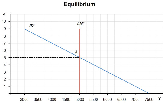
The graph is entitled “Equilibrium”. The vertical axis is labeled “e”, or the exchange rate, with values from 1 to 10 in single increments. The horizontal axis is labeled “Y”, which is the output, with values ranging from 3000 to 7500 in increments of 500. The LM curve is a vertical line at the value 5000. The IS curve is a downward sloping line that intersects the horizontal axis at 7500.  The point where the LM and IS curves intersect is the equilibrium and is labeled A. This point corresponds to an “e” of 5 and a “Y” value of 5000.

Review Chapter 13 pages 369-373, along with Figures 13-1, 13-2, and 13-3, for a discussion of how to derive the IS* curve and LM* curve, and how to use them to determine equilibrium for the economy.

Calculate the equilibrium exchange rate, level of income, and net exports.

The equilibrium exchange rate, ε, = .

The equilibrium level of income, Y, = .

The equilibrium level of net exports, NX, = .

Review Chapter 13 pages 369-373, along with Figures 13-1, 13-2, and 13-3, for a discussion of how to derive the IS* curve and LM* curve, and how to use them to determine equilibrium for the economy.

A small open economy is described by the following equations:

C = 300 +.8 (YT)

I = 900 – 50 r

NX = 500 – 100 ε

M/P = Y – 125 r

G = 1000

T = 1000

M = 8000

P = 2

r* = 8

Assume a floating exchange rate. Calculate what happens to the exchange rate, the level of income, net exports, and the money supply if the government reduces its spending by 100.

The exchange rate, ε, declines to .

The level of income, Y, is unchanged at .

The level of net exports, NX, rises to .

Money supply, M, is unchanged at .
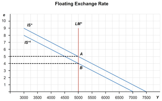
Review Chapter 13 pages 369-373, along with Figure 13-4, for a discussion of how changes in government purchases affect the economy in the Mundell-Fleming model under floating exchange rates.

The graph is entitled “Floating Exchange Rate”. The vertical axis is labeled “e”, or the exchange rate, with values from 1 to 10 in single increments. The horizontal axis is labeled “Y”, or the output, with values ranging from 3000 to 7500 in increments of 500.  The LM curve is a vertical line at the value 5000. The initial IS curve is a downward sloping line that intersects the horizontal axis at 7500. The point where the LM curve and the IS curve intersects is labeled A, and corresponds to an “e” of 5 and a “Y” value of 5000.   The new IS curve intersects the horizontal axis at 7000. The point where the LM curve and the new IS curve intersects is labeled B, and corresponds to an “e” of 4 and a “Y” value of 5000.

A small open economy is described by the following equations:

C = 300 +.8 (YT)

I = 900 – 50 r

NX = 500 – 100 ε

M/P = Y – 125 r

G = 1000

T = 1000

M = 8000

P = 2

r* = 8.

Now assume a fixed exchange rate. Calculate what happens to the exchange rate, the level of income, net exports, and the money supply if the government reduces its spending by 100.

The exchange rate, ε, is unchanged at .

The level of income, Y, declines to .

The level of net exports, NX, is unchanged at .

Money supply, M, declines to .

Review Chapter 13 pages 377-381, along with Figure 13-7, for a discussion of the Mundell-Fleming model under fixed exchange rates. See also the Case Study entitled, “The International Gold Standard.” Review Chapter 13 pages 380-382, along with Figure 13-8, for a discussion of how changes in government purchases affect the economy in the Mundell-Fleming model under fixed exchange rates.

The graph is entitled “Fixed Exchange Rate”. The vertical axis is labeled “e”, or the exchange rate, with values from 1 to 10 in single increments. The horizontal axis is labeled “Y”, or the output, with values ranging from 3000 to 7500 in increments of 500.  The graph shows the initial and new IS and LM curves.   The initial IS curve is a downward sloping line that intersects the horizontal axis at 7500.  The new IS curve intersects the horizontal axis at 7000.   The initial LM curve is a vertical line at the value 5000. The new LM curve is a vertical line at the value 4500.   The point where the initial IS and LM curves intersect is labeled A, and corresponds to an “e” of 5 and a “Y” value of 5000.   The point where the new IS curve and the initial LM curves intersects is labeled B, and corresponds to an “e” of 4 and a “Y” value of 5000.   The point where the new IS and LM curves intersect is labeled C, and corresponds to an “e” of 5 and a “Y” value of 4500.