Chapter 2. Laboratory Techniques

Exercise 1. Pipettes and Pipetting

Materials

Flask with water

10-mL serological pipette

Rack with eight culture tubes

Blue pi-pump

Practice cards with circles

Green pi-pump

p 100 micropipette

p 1000 micropipette

1-mL serological pipette

Example volumetric, Mohr, transfer and Pasteur pipets

PROCEDURE

Sample Pipettes (Work in Groups of 2)

Familiarize yourself with the following types of pipettes: volumetric, Mohr, serological, Pasteur

and transfer.

Pipetting Practice (Work in Groups of 2): Serological Pipettes

Using the appropriate serological pipette and pi-pump (1-mL pipette with blue pi-pump or 10-mL pipette with green pi-pump), dispense the following amounts of water into the test tubes:

Compare the volumes in each tube with the tubes your partner filled to make sure they match. If the volumes do not match, then empty the tubes back into the flask and repeat the exercise.

Clean-Up Procedure

1. Empty the water from the test tubes back into the flask.

2. Return the test tubes upside down to the rack to drain (four tubes per side).

3. Return pi-pumps to the basket and the pipettes to the jar. Make sure the neoprene gasket of the pi-pump did not come off and remains attached to the pipette!

Pipetting Practice (Work in Groups of 2): Micropipettes

1. Familiarize yourself with the two stops of the plunger. Be gentle.

2. Set the micropipette to the desired volume indicated on the practice card. Do not dial the volume adjustment knob out of range.

3. Place a disposable tip onto the end of the micropipette.

4. Draw up the desired volume of water and dispense it in the center of the appropriate circle on the practice card. The water should form a bead and exactly fill the circle.

5. Repeat steps 2-5 for each volume on the practice card.

Clean-Up Procedure

1. Return the micropipettes to the basket on the front table.

2. Discard tips in the beaker on the bench.

3. Discard practice cards and empty microcentrifuge tubes in the trash.

Exercise 2. Spectrometry (Work in Groups of 2)

Materials

PROCEDURE

1. Turn on the spectrometer by holding the power button on the right side for about three seconds or until the LED lights start to flash (see Figure 1-5).

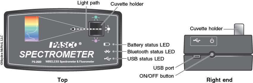
2. Plug the spectrometer into the computer via the USB cable (see Figure 1-5). To wirelessly connect to the spectrometer with a personal laptop or tablet, add a device in the Bluetooth settings and select the spectrometer that matches with the ID # on the bottom of the instrument.

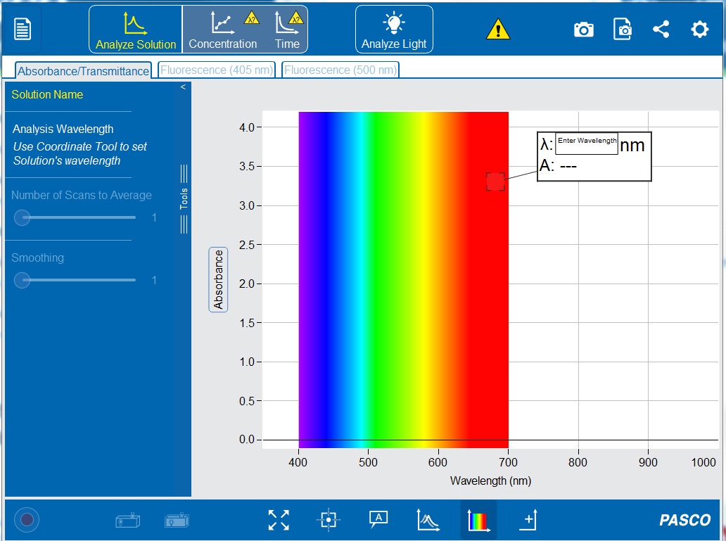
3. Open the PASCO Spectrometry app by clicking the icon . This should now show the initial screen of the PASCO Spectrometry display (see Figure 1-6) on your computer or tablet.

4. After a few seconds, the ‘Connection Status’ symbols on the top toolbar should turn from to . Click the circle to check that the ID # on the bottom of the spectrometer matches the display on your computer or tablet. If connecting wirelessly, a ‘Sensor Not Found’ error should pop up. Click . Select the spectrometer with the corresponding ID # and click . If a connection error does not pop up, click on the top toolbar.

5. Make sure the “Absorbance/Transmittance” tab is open on the top toolbar and the “Analyze Solution” setting is selected.

6. Wipe the blank cuvette with a Kimwipe and gently insert it into the cuvette holder. The cuvette should fit snugly. Do not remove the parafilm from the top of the cuvettes!

7. On the bottom toolbar, click “Calibrate Dark” to calibrate the spectrometer with the light turned off. A progress bar should appear, and after the calibration is complete, a check mark should appear.

8. Wait one to two minutes to allow the light source to warm up, then click “Calibrate Reference” to calibrate the spectrometer to the blank solution with the light on.

9. On the bottom toolbar, click “Start Record” . The symbol will change to the “Stop Record” icon and a horizontal line should appear at 0.0 ODU, indicating the spectrometer was properly calibrated. Tiny peaks in the line show noise, but if there are major peaks, repeat steps 7 and 8 to recalibrate the spectrometer.

10. In the “Enter Wavelength” box on the display (see Figure 1-6) type 510 nm to set the wavelength to 510 nanometers. If the white Enter Wavelength box is not already displayed on the graph, click the “Add Coordinate Tool” on the bottom toolbar. The coordinate tool can also be manually moved to set a wavelength.

11. Click to set the wavelength. A vertical line should appear on the graph at 510 nm, and the white box should now display the wavelength (λ) and the absorbance value (A).

12. Remove the blank cuvette from the spectrometer and return it to the rack.

13. Wipe the first sample cuvette, Solution A, with a Kimwipe and insert it into the cuvette holder. Instead of a straight line at 0.0 ODU, an absorbance spectrum should be visible on the graph.

14. You can increase the display size of the graph by clicking the “Scale to Fit” on the bottom toolbar or by clicking on the axes and dragging them to manually adjust the view.

15. On the bottom toolbar click the “Stop Record” . The symbol will return to the “Start Record” again.

16. To edit the name of the sample, click and then change the name.

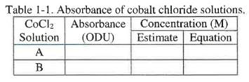
17. Record the absorbance value for the first sample in Table 1-1, and then remove the first sample cuvette.

18. Wipe and insert the second sample cuvette, Solution B. Click ‘Record’. The vertical line at 510 nm and the white box with the wavelength (λ) and the absorbance value (A) should already be on the graph.

19. Click ‘Record’ again to stop collecting data, and edit the name of the sample.

20. Enter the absorbance value for the second sample in Table 1-1, and then remove the second sample cuvette.

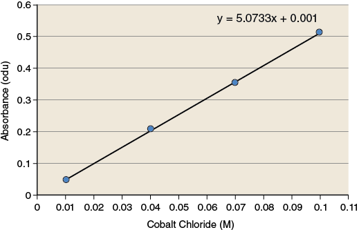
21. Use the standard curve to convert the absorbance values to concentrations by first estimating with a ruler and then using the equation to calculate more precise values. Record both values in Table 1-1.

After collecting data, explore the other options in the PASCO Spectrometry app that will be utilized during the semester.

22. To compare the absorbance spectra of the two samples, click “Show Comparison Mode” on the bottom toolbar to overlay the two graphs.

23. To take a picture of the graph, click “Take Journal Snapshot” on the top toolbar. When the image appears, click the download icon in the bottom left corner to save a .PNG file.

24. To record the absorbance of a sample over time, click the “Time” icon on the top toolbar. Next, on the bottom toolbar, click “Show Linear Fit” to display the best fit line. Since the absorbance should be constant for the sample, the line should be roughly horizontal. Lab 2 will explore change in absorbance over time.

25. To save an experiment or to open a new experiment, click “Experiment Options” on the top toolbar. Note: Anything saved to the lab computer will be deleted so anything you want to keep must be saved or sent to another device.

Clean-Up Procedure

1. Turn off the spectrometer by holding the power button.

2. Close the PASCO Spectrometry app. Leave the lab computer on.

3. Return the cuvettes to the rack.

4. Return the rulers to the jar.

Concentration Determination

The observations you have made during this exercise measure how much light is absorbed by the solution. These observations must be converted to values that have more relevance (concentration of product) because reaction rates are often expressed as changes in the concentration of product over time. To make these conversions you will use a standard curve. A standard curve is a graph relating a measured quantity to concentration of the substance of interest in “known” samples. The standard curve plots assayed quantity (on the y-axis) vs. concentration (on the x-axis). Such a curve can be used to determine concentrations of the substance in “unknown” samples. Using the standard curve for cobalt chloride shown in Figure 1-7, determine the concentration of CoCl₂ for the two sample solutions.

Record the values for the concentration of cobalt chloride for each of the sample solutions in your lab notebook.

Post-Lab Quiz

Proceed to the Post-Lab Quiz