Chapter 2. EVOLUTION I—POPULATION GENETICS
Since evolution is difficult, if not impossible, to observe in a 3-hour laboratory period, we will simulate the evolutionary process in different ways. You will use a benchtop simulation method in exercise 1 and the PopG program for four different scenarios in exercise 2 to depict changes in allele frequencies over time. This will give you the adequate practice so you can then develop a simulation of your own.
Exercise 1. Benchtop Bean Evolution Simulation
General Purpose
Conceptual
- Define evolution as it is defined by biologists and be able to describe how the components relate to experiments testing the concept of evolution.
- Define the term gene pool and explain how it relates to the concept of evolution.
- Gain an understanding of the concept of genetic equilibrium and the conditions required for it to occur.
- Gain an understanding of the relationship between genetic equilibrium and evolution.
- Gain an understanding of the Hardy-Weinberg equation and how it relates to population evolution.
- Gain an understanding of the impact of selection, mutation, and population size.
Procedural
- Be able to use the Hardy-Weinberg equation to calculate allele frequencies.
- Be able to graph the data obtained in this experiment, including a figure legend, and be able to descrie any trends in the data.
Materials per Student Group (2 students)
Mix of 50 white and 50 colored beans
5 dishes for beans, labeled: AA, Aa, aa, non-reproducing, and gene pool
Background Information
This exercise is a hands-on exercise to examine the allele frequency at one locus in a small population after a set number of generations in the presence of various amounts of selection, using physical representatives of two different alleles (black and white beans). This simple experiment can look at the forces that act in evolution. Given enough time and counting, the effect of mutation, migration, and fitness can all be examined. This pattern and concepts in this exercise are similar to the computer model which will be used for exercise 2.
PROCEDURE
Setup for the Simulation
- Prepare a table on a page of your lab notebook using Table 1-1 as a template.
Table 1-1. Allele frequency over ten generations of a population.
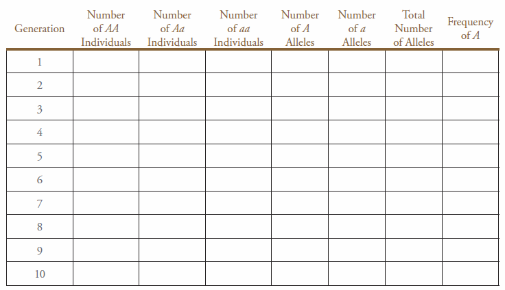
- Choose an organism and a trait with two phenotypes (e.g., pumpkins that are susceptible to powdery mildew when expressing one gene allele, versus the same species of pumpkin that is resistant to powdery mildew when expressing a different mutated allele of this gene). Record your choices in your lab notebook.
- Choose an environment that clearly favors one organism (e.g., field that has been infested with powdery mildew). Record your choice in your lab notebook.
- Choose which phenotype is determined by the dominant (A) allele. The white beans will represent this allele (A). Record your choice in your lab notebook.
- Determine the phenotype of the heterozygous individuals. This will be the same as the dominant (A) phenotype. Record your choice in your lab notebook.
- The fitness level for the favored phenotype is one. For the disadvantaged phenotype the fitness level is 0.5. This means 50% of the individuals will reproduce. Other individuals may survive to maturity, but since they do not reproduce, they do not contribute to the next generation. In exercise 2 you will use a computer program called PopG, which will allow you to look at thousands of generations. In that case a much smaller difference can be seen. Since in exercise 1 you are examining a small population and only ten generations, you will use a large disadvantage in order to see an effect and to overwhelm genetic drift. Record fitness level for each genotype in your lab notebook.
Benchtop Simulation
Generation 1
- Randomly select 50 individuals (two beans per each individual) and place individuals in correct genotype: homozygous dominant (2 white beans) in the AA dish, heterozygous (1 white bean and 1 colored bean) in the Aa dish, and homozygous recessive (2 colored beans) in the aa dish.
- Record the number of individuals of each genotype and total number of each of the alleles. The number of a and A alleles will each be approximately 50 for generation 1.
- Remove the homozygous individuals that will not successfully reproduce by placing one half of the non-reproducing genotype beans into the non-reproducing dish.
- If the heterozygous individuals are also selected against, then remove the beans (one of each type) for one half of these individuals and place the removed beans in the non-reproducing dish.
- Pool the beans representing the remaining reproducing alleles to generate the next generation.
Subsequent Generations
- Using the pooled beans from the previous generation, randomly select individuals and place individuals in the correct genotype.
- Repeat steps 2–5 from generation 1 for each subsequent generation, being sure to record the number of individuals for each genotype and the total number of each of the alleles in the table in your lab notebook.
- Stop once one of the alleles is fixed or once you reach ten generations.
- Complete the table in your lab notebook by calculating the frequency of A.
- Prepare a graph on a separate page of your lab notebook showing the frequency of A vs. generation number.
Exercise 2. Introduction to PopG Program
Background Information
PopG is a population genetics simulation program which models one locus with two alleles. This is a simple program that can be used to investigate evolutionary processes. One aspect of a scientific theory like evolution is that a theory is testable. Population models that result from simulations like this can then be used to make testable predictions about experimental or real-life outcomes. The initial portion of this exercise is designed to familiarize you with the parameters within the program that can be manipulated. In the subsequent portions of the exercise, you will use the program to model evolution. The various parameters you will be exploring (fitness, migration rate, mutation rate) are the same as those that could be studied in exercise 1. Unlike exercise 1, very small differences in the parameters can show significant impact on the allele frequency because the computer can simulate thousands of generations. The final portion of the exercise involves modeling a real-life example chosen by you.
PROCEDURE
A. Initial Simulation
- Open program by clicking on the PopG icon.
- Select Run/New Run.
- To use default parameters, select OK. The results of 10 simulations will appear as 10 lines on the graph of dominate allele frequency versus generational time.
- Under the “run” menu, select continue and enter 900 generations to see the same run continue to 1,000 generations.
It is possible that you may see the A allele frequency go to zero during those 1,000 generations. Alternatively you may see the A allele frequency go to 1. If either of those things occur, what does it mean?
B. Control Simulation
- Select Run/New Run.
- Change number of populations evolving simultaneously to 1. Only one population will be simulated and shown as one line. This is not changing an experimental parameter; it is changing the number of experiments run simultaneously.
- Change population size to 10,000 and generations to run to 1,000. Use these parameters for all following runs. Run the program. This run will serve as the control for the subsequent runs in which various parameters will be changed.
Record your results in your lab notebook. What is the final P(A)?
Does P(A) go to one or zero? If so, after how many generations does this occur?
C. Effect of Varying Fitness Simulation
- Select Run/New Run.
- Change the fitness level of the AA genotype to 0.98 and run program.
Is the phenotype expressed by AA more or less able to survive compared to the others? Record your observations in your lab notebook.
D. Effect of Varying Allele Starting Frequency Simulation
- Select Run/New Run.
- Change the starting allele frequency to 0.9 while keeping the fitness level of the AA genotype at 0.98 and run the program.
What is the experimental variable in this experiment?
Record your observations in your lab notebook.
What are the control conditions?
E. Effect of Mutation Rate Simulation
- Select Run/New Run.
- Change the mutation from a to A to 0.01 while keeping the fitness level of the AA genotype at 0.98 and run the program. Record your observations in your lab notebook.
F. Effect of Migration Rate Simulation
- Select Run/New Run.
- Change mutations to 0.
- Change the migration rate between populations to 0.1 while keeping the fitness level of the AA genotype at 0.98.
- Set the number of populations evolving to 2. Run the program.
Which parameter, mutation or migration, alters the results the most? Record your observations in your lab notebook.
In order to attribute changes to a specific parameter, how many other parameters can you change in a comparison during a run of the program?
G. Independent Experiment Simulation
In this part of the lab you will choose one of the conditions from the preceding simulations to explore further. Select one of the conditions you will use and write your choice in your lab notebook. The simulation you select will be run 10 times with the same conditions for 10 replicates. Do a second set of 10 replicates using conditions that fulfill the Hardy-Weinberg conditions (no evolution expected) as a control.
- Select Run/New Run.
- Type in the settings you have chosen for this simulation.
- Make sure that the “number of simultaneously evolving populations” is set to “1.”
- Run the program. Record your observations in your lab notebook.
- To rerun the simulation using the same settings, go to the “Run” menu and pull down to “Restart.”
- To run a simulation using different settings go to the “Run” menu and pull down to “New Run.”
Record your observations in your lab notebook after each of the 10 runs.
Make the appropriate graph of your results in your lab notebook.
2.1 Exercise 3. Stock Plate Production
General Purpose
Procedural
- Create a stock bacteria plate for subsequent use in replica plating.
Materials per Student Group (2 students)
Petri dish with growth media
Disinfecting solution of 10% bleach
Micropipettor
Sterile pipette tips
Bacterial stock culture
PROCEDURE
If you have not done so, please view the video in the pre-lab dealing with the method for preparing a bacterial plate.
Please read the procedures carefully and copy them into your lab notebook to avoid contaminating your bacterial samples.
- Disinfect your work area by wiping the benchtop with the disinfectant solution (10% bleach).
- Label the bottom of a sterile Petri plate containing growth medium with your name and section number.
- Using a micropipettor with a sterile tip pipette, transfer the designated number of μL of the bacterial stock culture from a microcentrifuge tube onto the surface of the growth medium in your Petri dish. Your laboratory instructor will tell you the exact volume to transfer and will have the bacterial culture microcentrifuge tubes.
- Evenly spread the bacteria across the surface of the growth medium using a sterile cell spreader.
- Seal the edge of the Petri plate with Parafilm.
- After 20 minutes, invert the Petri plate. Your lab instructor will incubate the plates at 37°C for approximately 12 hours and then transfer the plates to the refrigerator for storage.
Post-Lab Quiz
Proceed to the Post-Lab Quiz