Chapter 2. ECOLOGY—OVERVIEW
Learning Objectives
General Purpose
Conceptual
- Be able to determine changes in the University Lake system based on various biotic and abiotic data.
- Be able to relate the data collected in the population growth experiment to the biology of the lake system.
Procedural
- Be able to properly graph and analyze data.
- Be able to properly communicate results to a scientific audience in both written and oral form.
General Purpose
Populations within an ecosystem grow and their growth is impacted by the ecosystem’s biotic and abiotic factors (either singly or in combinations). You have examined the impact a single factor can have on the growth of a population in a controlled setting. You have also measured biotic and abiotic factors in an ecosystem. The challenge now is to combine those aspects to address how information from a controlled experiment may be used to help understand what may be happening in an ecosystem where complex interactions are occurring.
To start the process of integrating the two separate experiments, answer the following two questions and write the answers in your laboratory notebook.
- What was your independent variable in the Chlamydomonas population ecology experiment?
- Given that it will be easier to write a cohesive paper including Chlamydomonas data and the lake system if the parameters studied are similar, what lake aquatic measurement could you write about?
- Determine the appropriate independent variable and dependent variable for the lake system data.
Discuss with your lab partners and your lab instructor how you will approach the integration of the two different experiments. Recognize that to do this effectively you may need to compare and contrast the data from different sites or from different time points (or both). To prepare for that type of analysis, answer the following questions with your partner using the compiled data sheets. Write the answers in your laboratory notebook.
- Are dissolved oxygen levels higher in the spring, summer, or fall?
- Would you expect to see more autotrophs present in the spring, summer, or fall based on this result?
- Are chlorophyll levels higher at sites where nitrite levels are higher? Explain possible reasons why or why not in terms of autotrophs and heterotrophs.
- The University Lake system has high levels of phosphate in the bottom sediment. Will this stimulate the growth of autotrophs or heterotrophs?
It has been stressed that good experiments only have one variable and all other factors are constant. This is achievable in the laboratory where most conditions can be controlled. However, this is not realistic in many settings where it is either impractical or impossible to control all of the conditions. In fact in some cases it may be important to observe what occurs when all conditions are not controlled.
In the lake system, multiple parameters of interest may change at the same time. It is possible that in some cases a change in one factor may result in, or be caused by, changes in another factor. Modeling of the data is required to find a possible correlation between two parameters. You will choose an “independent” and a “dependent” variable from the collected data set available from your instructor to match an alternative hypothesis in the format of: the “independent” variable changed the “dependent” variable. The data collected at the same time and place can be plotted as one point, e.g. temperature and respiration from College Lake in the spring of 2013 is one data point.
Averaging data points across years and lake systems is not as powerful statistical method as when conditions can be controlled strictly. It is better to plot as much data as possible as separate points and fit the data to a model. The simplest model is a linear relationship between two variables. If a linear relationship is found, it should be possible to predict future values for the dependent variable if you know the independent variable, e.g. if the temperature the lake rises, the oxygen production will rise in a predictable way. There are many other types of models in addition to linear ones (e.g., exponential, logarithmic, etc.) that can require larger data sets and more sophisticated mathematics.
Graphing programs typically will fit any set of points to a trend line. For a linear relationship a trend line following the equation y = mx + b, where m is the slope of the line and b is the y-intercept. In the simplest method for fitting a linear trend line to a set of data, the program minimizes the total difference between points above and below the estimated line. In general terms the line is describing in a mathematical way how a change in one variable effects a change in another variable. This correlation between the variables can be classified into three types:
- a positive correlation (X goes up and so does Y) and the slope of the line is positive
- a negative correlation (X goes up and Y goes down – also known as a reciprocal relationship) and slope of the lime is negative
- a zero correlation (increase or decrease in X has no clear impact on Y).
The type of correlation can be expressed as a mathematical value known as the correlation coefficient (R) that can vary between -1 to +1.
To assess the how well a group of data matches a linear model or trend line the square of the correlation coefficient (R2) can be used. R2 values can range between 0, no correlation, to 1, a perfect fit where all data points lie directly on the trend line. Different fields of research and various types of experiments require differing levels of correlation to support the alternative hypothesis. Discuss with your Instructor an R2 value that would be sufficient for supporting the alternative hypothesis.
The data for temperature (independent variable) vs respiration (dependent variable) can be potted and fitted with a trend line (see Figure 7-1).
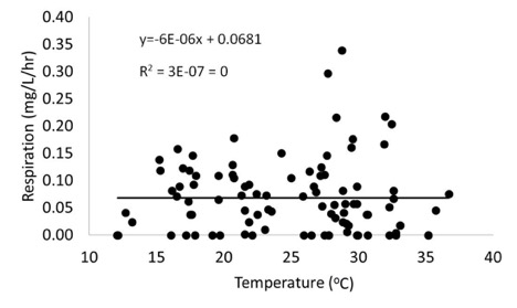
The equation for the line and the R2 value are shown in the graph. Since the R2 value equals zero in this case, one can clearly reject the alternative hypothesis. In the LSU lake system, temperature does influence respiration in an easily modeled way. More complex relationships may be found by non-linear modeling.
|
|
||||||||||