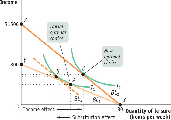
Figure19A-4Labour Supply Choice: The Indifference Curve Approach Point A, on BL₁, is Clive’s initial optimal choice. After a wage rate increase, his income and utility level increase: his new time allocation budget line is BL₂ and his new optimal choice is point C. This change can be decomposed into the substitution effect, the fall in the hours of leisure from point A to point S, and the income effect, the increase in the number of hours of leisure from point S to pointC. As shown here, the income effect dominates the substitution effect: the net result of an increase in the wage rate is an increase in the hours of leisure consumed and a decrease in the hours of labour supplied.