At the beginning of the last section, we used indifference curves to represent the preferences of Ingrid, whose consumption bundles consist of rooms and restaurant meals. Our next step is to show how to use Ingrid’s indifference curve map to find her utility-maximizing consumption bundle given her budget constraint, the fact that she must choose a consumption bundle that costs no more than her total income.

It’s important to understand how our analysis here relates to what we did in Chapter 10. We are not offering a new theory of consumer behaviour in this appendix—just as in Chapter 10, consumers are assumed to maximize total utility. In particular, we know that consumers will follow the optimal consumption rule from Chapter 10: the optimal consumption bundle lies on the budget line, and the marginal utility per dollar is the same for every good in that bundle.

But as we’ll see shortly, we can derive this optimal consumer behaviour in a somewhat different way—a way that yields deeper insights into consumer choice.

The Marginal Rate of Substitution The first element of our approach is a new concept, the marginal rate of substitution. The essence of this concept is illustrated in Figure 10A-5.

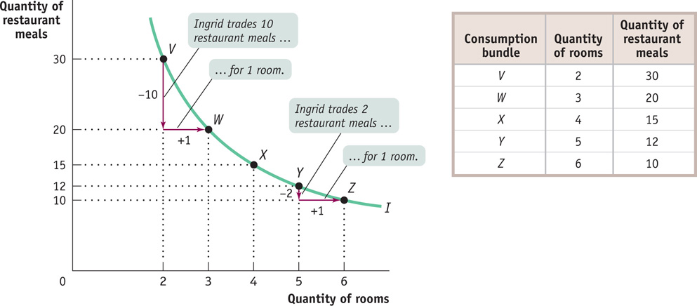
Recall from the last section that for most goods, consumers’ indifference curves are downward sloping and strictly convex. Figure 10A-5 shows such an indifference curve. The points labelled V, W, X, Y, and Z all lie on this indifference curve—that is, they represent consumption bundles that yield Ingrid the same level of total utility. The table accompanying the figure shows the components of each of the bundles. As we move along the indifference curve from V to Z, Ingrid’s consumption of housing steadily increases from 2 rooms to 6 rooms, her consumption of restaurant meals steadily decreases from 30 meals to 10 meals, and her total utility is kept constant. As we move down such a strictly convex indifference curve, then, Ingrid is trading more of one good in place of less of the other, with the terms of that trade-off—the ratio of additional rooms consumed to restaurant meals sacrificed—chosen to keep her total utility constant.

Notice that the quantity of restaurant meals that Ingrid is willing to give up in return for an additional room changes along the indifference curve. As we move from V to W, housing consumption rises from 2 to 3 rooms and restaurant meal consumption falls from 30 to 20—a trade-off of 10 restaurant meals for 1 additional room. But as we move from Y to Z, housing consumption rises from 5 to 6 rooms and restaurant meal consumption falls from 12 to 10, a trade-off of only 2 restaurant meals for an additional room.

To put it in terms of slopes, the slope of the indifference curve between V and W is –10: the change in restaurant meal consumption, –10, divided by the change in housing consumption, 1. Similarly, the slope of the indifference curve between Y and Z is –2. So the indifference curve gets flatter as we move down it to the right—that is, it has a strictly convex shape, one of the four properties of an indifference curve for ordinary goods.

Why does the trade-off change in this way? Let’s think about it intuitively, and then work through it more carefully. When Ingrid moves down along her indifference curve, whether from V to W or from Y to Z, she gains utility from her additional consumption of housing but loses an equal amount of utility from her reduced consumption of restaurant meals. But at each step, the initial position from which Ingrid begins is different. At V, Ingrid consumes only a small quantity of rooms; because of diminishing marginal utility, her marginal utility per room at that point is high. At V, then, an additional room adds a lot to Ingrid’s total utility. But at V she already consumes a large quantity of restaurant meals, so her marginal utility of restaurant meals is low at that point. This means that, at V, it takes a large reduction in her quantity of restaurant meals consumed to offset the increased utility she gets from the extra room of housing.

At Y, in contrast, Ingrid consumes a much larger quantity of rooms and a much smaller quantity of restaurant meals than at V. This means that an additional room adds fewer utils, and a restaurant meal forgone costs more utils, than at V. So Ingrid is willing to give up fewer restaurant meals in return for another room of housing at Y (where she gives up 2 meals for 1 room) than she is at V (where she gives up 10 meals for 1 room).

Now let’s express the same idea—that the trade-off Ingrid is willing to make depends on where she is starting from—by using a little math. We do this by examining how the slope of the indifference curve changes as we move down it. Moving down along the indifference curve—reducing restaurant meal consumption and increasing housing consumption—will produce two opposing effects on Ingrid’s total utility: lower restaurant meal consumption will reduce her total utility, but higher housing consumption will raise her total utility. And since we are moving down along the indifference curve, these two effects must exactly cancel out:

Along the indifference curve:

or, rearranging terms,

Along the indifference curve:

Let’s now focus on what happens as we move only a short distance down the indifference curve, trading off a small increase in housing consumption in place of a small decrease in restaurant meal consumption. Following our notation from Chapter 10, let’s use MU_R and MU_M to represent the marginal utility of rooms and restaurant meals, respectively, and ΔQ_R and ΔQ_M to represent the changes in room and meal consumption, respectively. In general, the change in total utility caused by a small change in consumption of a good is equal to the change in consumption multiplied by the marginal utility of that good. This means that we can calculate the change in Ingrid’s total utility generated by a change in her consumption bundle using the following equations:

and

So we can write Equation 10A-2 in symbols as:

Along the indifference curve:

Note that the left-hand side of Equation 10A-5 has a minus sign; it represents the loss in total utility from decreased restaurant meal consumption. This must equal the gain in total utility from increased room consumption, represented by the right-hand side of the equation.

What we want to know is how this translates into the slope of the indifference curve. To find the slope, we divide both sides of Equation 10A-5 by ΔQ_R, and again by –MU_M, in order to get the ΔQ_M, ΔQ_R terms on one side and the MU_R, MU_M terms on the other. This results in:

Slope along the indifference curve:

The left-hand side of Equation 10A-6 is the slope of the indifference curve; it is the rate at which Ingrid is willing to trade rooms (the good on the horizontal axis) in place of restaurant meals (the good on the vertical axis) without changing her total utility level. The right-hand side of Equation 10A-6 is minus the ratio of the marginal utility of rooms to the marginal utility of restaurant meals—that is, the ratio of what she gains from one more room to what she gains from one more meal.

Putting all this together, we see that Equation 10A-6 shows that, along the indifference curve, the quantity of restaurant meals Ingrid is willing to give up in return for a room, ΔQ_M/ΔQ_R, is exactly equal to minus the ratio of the marginal utility of a room to that of a meal, –MU_R/MU_M. Only when this condition is met will her total utility level remain constant as she consumes more rooms and fewer restaurant meals.

Economists have a special name for the ratio of the marginal utilities found in the right-hand side of Equation 10A-6: it is called the marginal rate of substitution, or MRS, of rooms (the good on the horizontal axis) in place of restaurant meals (the good on the vertical axis). That’s because as we slide down Ingrid’s indifference curve, we are substituting more rooms in place of fewer restaurant meals in her consumption bundle. As we’ll see shortly, the marginal rate of substitution plays an important role in finding the optimal consumption bundle.

Recall that indifference curves get flatter as you move down them to the right. The reason, as we’ve just discussed, is diminishing marginal utility: as Ingrid consumes more housing and fewer restaurant meals, her marginal utility from housing falls and her marginal utility from restaurant meals rises. So her marginal rate of substitution, which is equal to minus the slope of her indifference curve, falls as she moves down along the indifference curve.

The flattening of indifference curves as you slide down them to the right—which reflects the same logic as the principle of diminishing marginal utility—is known as the principle of diminishing marginal rate of substitution. It says that an individual who consumes only a little bit of good A and a lot of good B will be willing to trade off a lot of B in return for one more unit of A; an individual who already consumes a lot of A and not much B will be less willing to make that trade-off.

We can illustrate this point by referring back to Figure 10A-5. At point V, a bundle with a high proportion of restaurant meals to rooms, Ingrid is willing to forgo 10 restaurant meals in return for 1 room. But at point Y, a bundle with a low proportion of restaurant meals to rooms, she is willing to forgo only 2 restaurant meals in return for 1 room.

From this example we can see that, in Ingrid’s utility function, rooms and restaurant meals possess the two additional properties that characterize ordinary goods. Ingrid requires additional rooms to compensate her for the loss of a meal, and vice versa; so her indifference strictly curves for these two goods slope downward. And her indifference curves are strictly convex: the slope of her indifference curve—minus the marginal rate of substitution—becomes flatter as we move down it. In fact, an indifference curve is strictly convex only when it has diminishing marginal rate of substitution—these two conditions are equivalent.

With this information, we can define ordinary goods, which account for the great majority of goods in any consumer’s utility function. A pair of goods are ordinary goods in a consumer’s utility function if they possess two properties: the consumer requires more of one good to compensate for less of the other, and the consumer experiences a diminishing marginal rate of substitution when substituting one good in place of the other.

Next we will see how to determine Ingrid’s optimal consumption bundle using indifference curves.

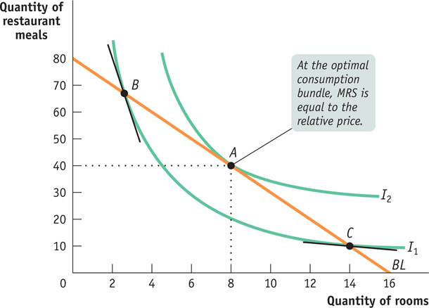
The Tangency Condition Now let’s put some of Ingrid’s indifference curves on the same diagram as her budget line, to illustrate an alternative way of representing her optimal consumption choice. Figure 10A-6 shows Ingrid’s budget line, BL, when her income is $2400 per month, housing costs $150 per room each month, and restaurant meals cost $30 each. What is her optimal consumption bundle?

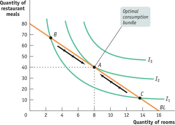
To answer this question, we show several of Ingrid’s indifference curves: I₁, I₂, and I₃. Ingrid would like to achieve the total utility level represented by I₃, the highest of the three curves, but she cannot afford to because she is constrained by her income: no consumption bundle on her budget line yields that much total utility. But she shouldn’t settle for the level of total utility generated by B, which lies on I₁: there are other bundles on her budget line, such as A, that clearly yield higher total utility than B.

In fact, A—a consumption bundle consisting of 8 rooms and 40 restaurant meals per month—is Ingrid’s optimal consumption choice. The reason is that A lies on the highest indifference curve Ingrid can reach given her income.

At the optimal consumption bundle A, Ingrid’s budget line just touches the relevant indifference curve—the budget line is tangent to the indifference curve. This tangency condition between the indifference curve and the budget line applies to the optimal consumption bundle when the indifference curves have the typical strictly convex shape: at the optimal consumption bundle, the budget line just touches—is tangent to—the indifference curve.

To see why, let’s look more closely at how we know that a consumption bundle that doesn’t satisfy the tangency condition can’t be optimal. Re-examining Figure 10A-6, we can see that the consumption bundles B and C are both affordable because they lie on the budget line. However, neither is optimal. Both of them lie on the indifference curve I₁, which cuts through the budget line at both points. But because I₁ cuts through the budget line, Ingrid can do better: she can move down the budget line from B or up the budget line from C, as indicated by the arrows. In each case, this allows her to get onto a higher indifference curve, I₂, which increases her total utility.

Ingrid cannot, however, do any better than I₂: any other indifference curve either cuts through her budget line or doesn’t touch it at all. And the bundle that allows her to achieve I₂ is, of course, her optimal consumption bundle.

The Slope of the Budget Line Figure 10A-6 shows us how to use a graph of the budget line and the indifference curves to find the optimal consumption bundle, the bundle at which the budget line and the indifference curve are tangent. But rather than rely on drawing graphs, we can determine the optimal consumption bundle by using a bit of math. As you can see from Figure 10A-6, at A, the optimal consumption bundle, the budget line and the indifference curve have the same slope. Why? Because two curves can only touch each other if they have the same slope at their point of tangency. Otherwise, they would cross each other somewhere. And we know that if we are on an indifference curve that crosses the budget line (like I₁ in Figure 10A-6), we can’t be on the indifference curve that contains the optimal consumption bundle (like I₂).

So we can use information about the slopes of the budget line and the indifference curve to find the optimal consumption bundle. To do that, we must first analyze the slope of the budget line, a fairly straightforward task. We know that Ingrid will get the highest possible utility by spending all of her income and consuming a bundle on her budget line. So we can represent Ingrid’s budget line, the consumption bundles available to her when she spends all of her income, with the equation:

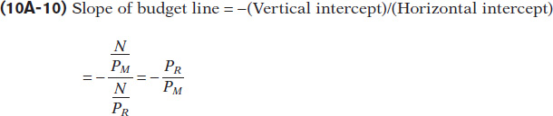
where N stands for Ingrid’s income. To find the slope of the budget line, we divide its vertical intercept (where the budget line hits the vertical axis) by its horizontal intercept (where it hits the horizontal axis). The vertical intercept is the point at which Ingrid spends all her income on restaurant meals and none on housing (that is, Q_R = 0). In that case the number of restaurant meals she consumes is:

At the other extreme, Ingrid spends all her income on housing and none on restaurant meals (so that Q_M = 0). This means that at the horizontal intercept of the budget line, the number of rooms she consumes is:

Now we have the information needed to find the slope of the budget line. It is:

Notice the minus sign in Equation 10A-10; it’s there because the budget line slopes downward. The quantity P_R/P_M is known as the relative price of rooms in terms of restaurant meals, to distinguish it from an ordinary price in terms of dollars. Because buying one more room requires Ingrid to give up P_R/P_M quantity of restaurant meals, or 5 meals, we can interpret the relative price P_R/P_M as the rate at which a room trades for restaurant meals in the market; it is the price—in terms of restaurant meals—Ingrid has to “pay” to get one more room.

Looking at this another way, the slope of the budget line—minus the relative price—tells us the opportunity cost of each good in terms of the other. The relative price illustrates the opportunity cost to an individual of consuming one more unit of one good in terms of how much of the other good in his or her consumption bundle must be forgone. This opportunity cost arises from the consumer’s limited resources—his or her limited budget. It’s useful to note that Equations 10A-8, 10A-9, and 10A-10 give us all the information we need about what happens to the budget line when relative price or income changes. From Equations 10A-8 and 10A-9 we can see that a change in income, N, leads to a parallel shift of the budget line: both the vertical and horizontal intercepts will shift. That is, how far out the budget line is from the origin depends on the consumer’s income. If a consumer’s income rises, the budget line moves outward. If the consumer’s income shrinks, the budget line shifts inward. In each case, the slope of the budget line stays the same because the relative price of one good in terms of the other does not change.

In contrast, a change in the relative price P_R/P_M will lead to a change in the slope of the budget line. We’ll analyze these changes in the budget line and how the optimal consumption bundle changes when the relative price changes or when income changes in greater detail later in the appendix.

Prices and the Marginal Rate of Substitution Now we’re ready to bring together the slope of the budget line and the slope of the indifference curve to find the optimal consumption bundle. From Equation 10A-6, we know that the slope of the indifference curve at any point is equal to minus the marginal rate of substitution:

As we’ve already noted, at the optimal consumption bundle the slope of the budget line and the slope of the indifference curve are equal. We can write this formally by putting Equations 10A-10 and 10A-11 together, which gives us the relative price rule for finding the optimal consumption bundle:

At the optimal consumption bundle:

That is, at the optimal consumption bundle, the marginal rate of substitution between any two goods is equal to the ratio of their prices. Or to put it in a more intuitive way, at Ingrid’s optimal consumption bundle, the rate at which she would trade a room in exchange for having fewer restaurant meals along her indifference curve, MU_R/MU_M, is equal to the rate at which rooms are traded for restaurant meals in the market, P_R/P_M.

What would happen if this equality did not hold? We can see by examining Figure 10A-7. There, at point B, the slope of the indifference curve, –MU_R/MU_M, is greater in absolute value than the slope of the budget line, −P_R/P_M. This means that, at B, Ingrid values an additional room in place of meals more than it costs her to buy an additional room and forgo some meals. As a result, Ingrid would be better off moving down along her budget line toward A, consuming more rooms and fewer restaurant meals—and because of that, B could not have been her optimal bundle! Likewise, at C, the slope of Ingrid’s indifference curve is less than the slope of the budget line. The implication is that, at C, Ingrid values additional meals in place of a room more than it costs her to buy additional meals and forgo a room. Again, Ingrid would be better off moving up along her budget line—consuming more restaurant meals and fewer rooms—until she reaches A, her optimal consumption bundle.

But suppose that we do the following transformation to the last term of Equation 10A-12: divide both sides by P_R and multiply both by MU_M. Then the relative price rule becomes (from Chapter 10, Equation 10-3):

Optimal consumption rule:

So using either the optimal consumption rule (from Chapter 10) or the relative price rule (from this appendix), we find the same optimal consumption bundle. At the optimal consumption bundle, not only do Equations 10A-12 and 10A-13 hold, but also the budget constraint Equation 10A-7 must hold, since the bundle is on the budget line. So the budget constraint and the indifference curves have the same slope at the optimal consumption bundle.

Preferences and Choices Now that we have seen how to represent optimal consumption choice in an indifference curve diagram, we can turn briefly to the relationship between consumer preferences and consumer choices.

When we say that two consumers have different preferences, we mean that they have different utility functions. This in turn means that they will have indifference curve maps with different shapes. And those different maps will translate into different optimal consumption choices, even among consumers with the same income and who face the same prices.

To see this, suppose that Ingrid’s friend Lars also consumes only housing and restaurant meals. However, Lars has a stronger preference for restaurant meals and a weaker preference for housing. This difference in preferences is shown in Figure 10A-8, which shows two sets of indifference curves: panel (a) shows Ingrid’s preferences and panel (b) shows Lars’s preferences. Note the difference in their shapes.

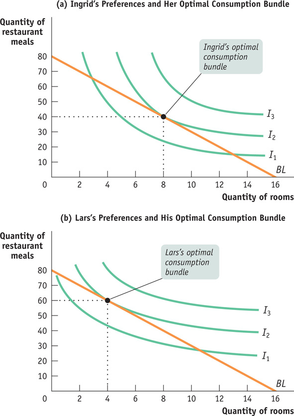
Suppose, as before, that rooms cost $150 per month and restaurant meals cost $30. Let’s also assume that both Ingrid and Lars have incomes of $2400 per month, giving them identical budget lines. Nonetheless, because they have different preferences, they will make different optimal consumption choices, as shown in Figure 10A-8. Ingrid will choose 8 rooms and 40 restaurant meals; Lars will choose 4 rooms and 60 restaurant meals.