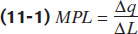
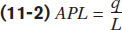
In the chapter, we defined the marginal product of labour (MPL) and the average product of labour (APL):

Now, let’s turn to a firm’s costs of production. For any firm, the amount of capital employed in the production process (such as property, machinery, and equipment) is assumed to be constant in the short run. We also assume that the state of production technology is fixed. In the short run, the firm can only adjust the amount of labour employed, the variable input. Since the firm must pay both fixed costs (FC) and the variable cost (VC) of labour to produce its output, its total cost (TC) can be expressed in terms of labour:

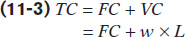
where w is the wage rate page for one unit of labour. For example, suppose the hourly wage at a bakery is $15 and the daily fixed costs total $2000. We can express the bakery’s total cost in terms of the number of hours of labour as:

TC = 2000 + 15 × L

A firm should be interested in minimizing its cost of production for a given level of output. Then, the problem becomes how to minimize TC, subject to q.

Recall, marginal cost, MC, is the additional cost incurred by producing an additional unit of output. We expressed it as the change in total cost divided by the change in output:

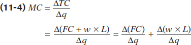
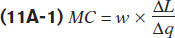
Since fixed costs do not change, ΔFC is zero. The wage is also constant, so the term w can be moved outside of the fraction:

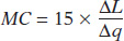
An example may make this algebra clearer. For the bakery, the change in total cost (TC = 2000 + 15 × L) can be separated into the change in the fixed cost ($2000) plus the change in the variable cost of $15 multiplied by the change in hours of labour. The fixed amount does not change by definition, and only the number of hours of labour changes. At the bakery, the marginal cost is:

Now go back and look at Equation 11-1. The fraction in the equations above is the inverse of ∆q divided by ∆L, the marginal product of labour. Therefore, we can rewrite marginal cost as:

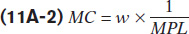
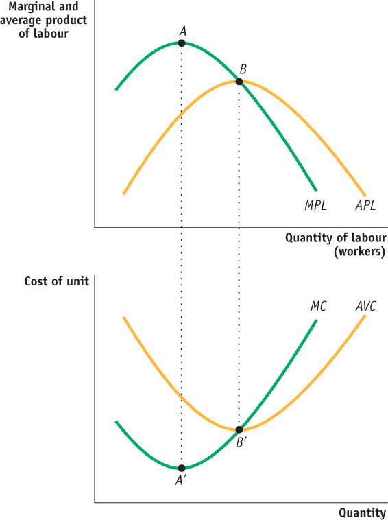
Now, it is clear that marginal cost falls when marginal product of labour rises; when the marginal product of labour falls, the marginal cost rises. Also, when marginal product is maximized, marginal cost reaches its minimum.

Discovering the inverse relationship between the average product of labour and average variable cost, AVC, is somewhat easier. In the chapter, we defined AVC as the variable cost per unit of output:

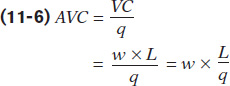
Since Equation 11-2 describes APL as q divided by L, we have another inverse relationship. We can rewrite the average variable cost as:

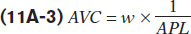
Now, you can clearly see the inverse relationship between these two concepts. When average product of labour rises, average variable costs falls; when average product of labour falls, average variable costs rises. When average product is maximized, average variable cost reaches its minimum. Figure 11A-1 summarizes these relationships geometrically.