A Key Concept: The Slope of a Curve
The slope of a line or curve is a measure of how steep or flat it is. The slope of a line is measured by “rise over run”—the change in the y-variable between two points on the line divided by the change in the x-variable between those same two points.
The slope of a curve is a measure of how steep or flat it is and indicates how sensitive the y-variable is to a change in the x-variable. In our example of outside temperature and the number of cans of pop a vendor can expect to sell, the slope of the curve would indicate how many more cans of pop the vendor could expect to sell with each 1 degree increase in temperature. Interpreted this way, the slope gives meaningful information. Even without numbers for x and y, it is possible to arrive at important conclusions about the relationship between the two variables by examining the slope of a curve at various points.
The Slope of a Linear Curve Along a linear curve the slope, or steepness, is measured by dividing the “rise” between two points on the curve by the “run” between those same two points. The rise is the amount that y changes, and the run is the amount that x changes. Here is the formula:
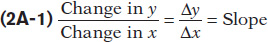
In the formula, the symbol Δ (the Greek uppercase delta) stands for “change in.” When a variable increases, the change in that variable is positive; when a variable decreases, the change in that variable is negative.
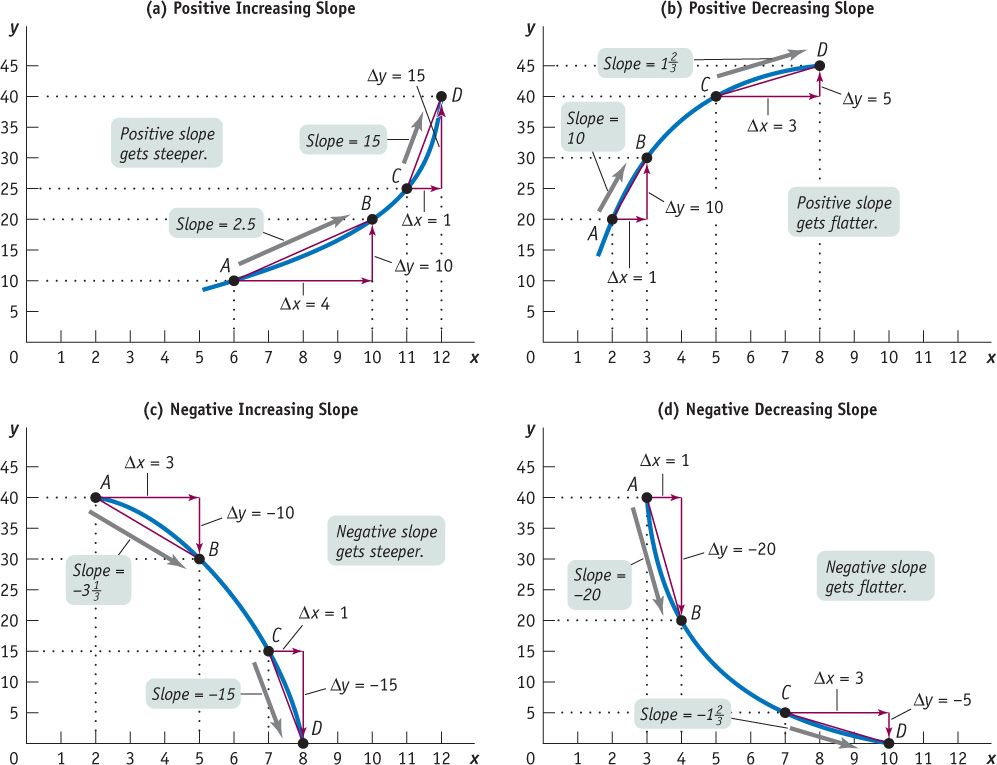
The slope of a curve is positive when the rise (the change in the y-variable) has the same sign as the run (the change in the x-variable). That’s because when two numbers have the same sign, the ratio of those two numbers is positive. The curve in panel (a) of Figure 2A-2 has a positive slope: along the curve, both the y-variable and the x-variable increase. The slope of a curve is negative when the rise and the run have different signs. That’s because when two numbers have different signs, the ratio of those two numbers is negative. The curve in panel (b) of Figure 2A-2 has a negative slope: along the curve, an increase in the x-variable is associated with a decrease in the y-variable.
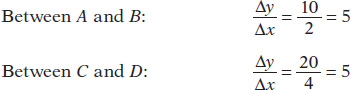
Figure 2A-3 illustrates how to calculate the slope of a linear curve. Let’s focus first on panel (a). From point A to point B the value of the y-variable changes from 25 to 20 and the value of the x-variable changes from 10 to 20. So the slope of the line between these two points is:
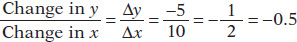
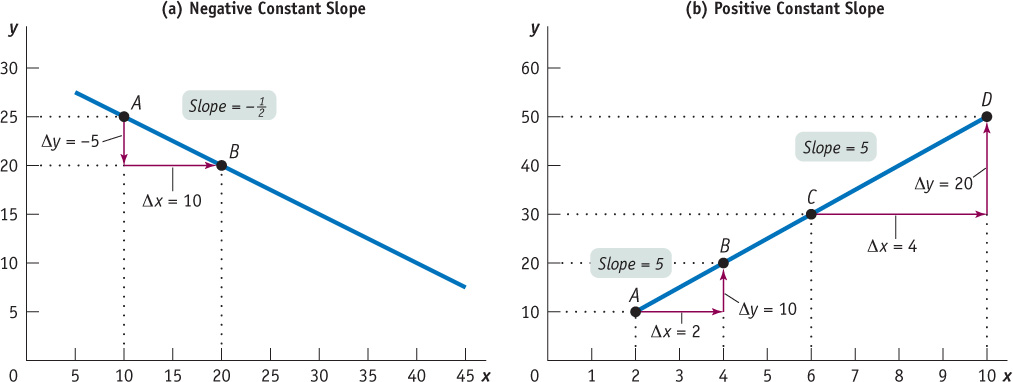
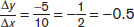 , where the negative sign indicates that the curve is downward sloping. In panel (b), the curve has a slope from A to B of
  . The slope from C to D is
  . The slope is positive, indicating that the curve is upward sloping. Furthermore, the slope between A and B is the same as the slope between C and D, making this a linear curve. The slope of a linear curve is constant: it is the same regardless of where it is measured along the curve.
Because a straight line is equally steep at all points, the slope of a straight line is the same at all points. In other words, a straight line has a constant slope. You can check this by calculating the slope of the linear curve between points A and B and between points C and D in panel (b) of Figure 2A-3.
Horizontal and Vertical Curves and Their Slopes When a curve is horizontal, the value of the y-variable along that curve never changes—
If a curve is vertical, the value of the x-variable along the curve never changes—
A vertical or a horizontal curve has a special implication: it means that the x-variable and the y-variable are unrelated. Two variables are unrelated when a change in one variable (the independent variable) has no effect on the other variable (the dependent variable). Or to put it a slightly different way, two variables are unrelated when the dependent variable is constant regardless of the value of the independent variable. If, as is usual, the y-variable is the dependent variable, the curve is horizontal. If the dependent variable is the x-variable, the curve is vertical.
A non-linear curve is one in which the slope is not the same between every pair of points.
The Slope of a Non-
 , and from C to D it is
  . The slope is positive and increasing; the curve gets steeper as you move to the right. In panel (b) the slope of the curve from A to B is
  , and from C to D it is
  . The slope is positive and decreasing; the curve gets flatter as you move to the right. In panel (c) the slope from A to B is
  , and from C to D it is
  . The slope is negative and increasing; the curve gets steeper as you move to the right. And in panel (d) the slope from A to B is
  , and from C to D it is
  . The slope is negative and decreasing; the curve gets flatter as you move to the right. The slope in each case has been calculated by using the arc method—
When we calculate the slope along these non-
The absolute value of a negative number is the value of the negative number without the minus sign.
The slopes of the curves in panels (c) and (d) are negative numbers. Economists often prefer to express a negative number as its absolute value, which is the value of the negative number without the minus sign. In general, we denote the absolute value of a number by two parallel bars around the number; for example, the absolute value of −4 is written as |−4| = 4. In panel (c), the absolute value of the slope steadily increases as you move from left to right. The curve therefore has negative increasing slope (i.e., the absolute value of the slope is increasing, so the curve is getting steeper). And in panel (d), the absolute value of the slope of the curve steadily decreases along the curve. This curve therefore has negative decreasing slope.
Calculating the Slope Along a Non-
The Arc Method of Calculating the Slope An arc of a curve is some piece or segment of that curve. For example, panel (a) of Figure 2A-4 shows an arc consisting of the segment of the curve between points A and B. To calculate the slope along a non-
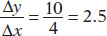
This means that the average slope of the curve between points A and B is 2.5.
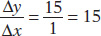
Now consider the arc on the same curve between points C and D. A straight line drawn through these two points increases along the x-axis from 11 to 12 (Δx = 1) as it increases along the y-axis from 25 to 40 (Δy = 15). So the average slope between points C and D is:
Therefore the average slope between points C and D is larger than the average slope between points A and B. These calculations verify what we have already observed—
The Point Method of Calculating the Slope The point method calculates the slope of a non-
 .
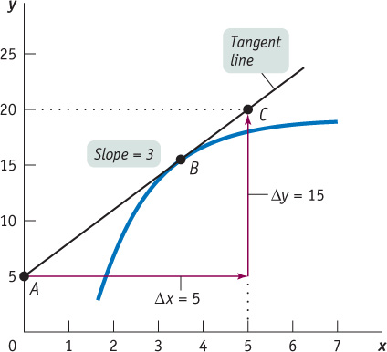
.A tangent line is a straight line that just touches, or is tangent to, a non-
You can see from Figure 2A-5 how the slope of the tangent line is calculated: from point A to point C, the change in y is 15 and the change in x is 5, generating a slope of:

By the point method, the slope of the curve at point B is equal to 3.
A natural question to ask at this stage is how to determine which method to use—
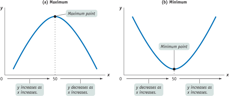
Maximum and Minimum Points The slope of a non-
Panel (a) of Figure 2A-6 illustrates a curve in which the slope changes from positive to negative as you move from left to right. When x is between 0 and 50, the slope of the curve is positive. At x equal to 50, the curve attains its highest point—
A non-
A non-
In contrast, the curve shown in panel (b) of Figure 2A-6 is U-