The income elasticity of demand measures how sensitive the demand curve is to changes in consumers’ incomes by measuring how far the demand curve parallel shifts along the quantity axis as consumers’ incomes change. More precisely, it measures the percentage change in quantity demand per percentage change in income. To examine income algebraically, we need to revisit the expanded version of Equation 3A-1 from Appendix 3A:

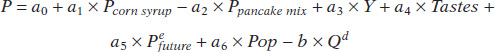
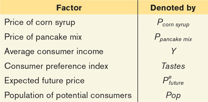
where P denotes the price, Q^d denotes the quantity, and the other terms are positive constants. Table 6A-1 summarizes the factors in this equation. For the income elasticity of demand, we are dealing with the Y term, average consumer income.

If we isolate Q^d as a function of the other terms, we get:

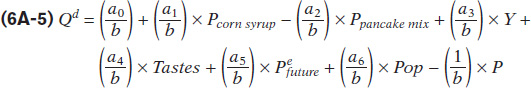
As we noticed in Equation 6A-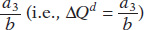1, according to Equation 6A-5, if the average consumer income increases by $1 (i.e., ΔY = 1), then the quantity demanded for maple syrup will increase by . Therefore, the ratio is equal to .

So, using the general demand curve given above, we get:

We know that b, Y, and Q^d are all positive, so a₃ determines whether the income elasticity of demand is positive or negative:

If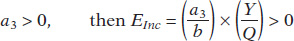

If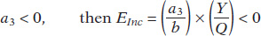

So if a₃ > 0, this good is a normal good (like maple syrup) because an increase in income results in an increase in demand. Similarly, if a₃ < 0, this good is an inferior good because an increase in income results in a decrease in demand.