12.3 The Industry Supply Curve
The industry supply curve shows the relationship between the price of a good and the total output supplied by the industry as a whole.
Why will an increase in the demand for organic tomatoes lead to a large price increase at first but a much smaller increase in the long run? The answer lies in the behaviour of the industry supply curve—the relationship between the price and the total output of an industry as a whole. The industry supply curve is what we referred to in earlier chapters as the supply curve or the market supply curve. But here we take some extra care to distinguish between the individual supply curve of a single firm and the supply curve of the industry as a whole.
As you might guess from the previous section, the industry supply curve must be analyzed in somewhat different ways for the short run and the long run. Let’s start with the short run.
The Short-Run Industry Supply Curve
Recall that in the short run the number of producers in an industry is fixed—
The short-run industry supply curve shows how the quantity supplied by an industry depends on the market price given a fixed number of producers.
Each of these 100 farms will have an individual short-
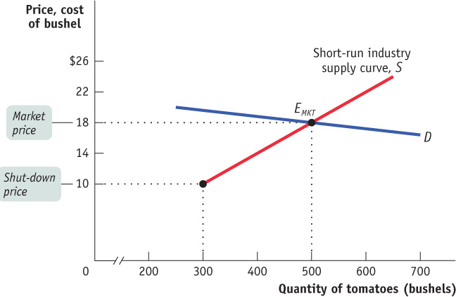
There is a short-run market equilibrium when the quantity supplied equals the quantity demanded, taking the number of producers as given.
The demand curve D in Figure 12-5 crosses the short-
The Long-Run Industry Supply Curve
Suppose that in addition to the 100 farms currently in the organic tomato business, there are many other potential producers. Suppose also that each of these potential producers would have the same cost curves as existing producers like Jennifer and Jason if it entered the industry.
In the long run, when will additional producers enter the industry? Whenever existing producers are making a profit—
What will happen as additional producers enter the industry? Clearly, the quantity supplied at any given price will increase. The short-
Figure 12-6 illustrates the effects of this chain of events on an existing firm and on the market; panel (a) shows how the market responds to entry, and panel (b) shows how an individual existing firm responds to entry. (Note that these two graphs have been rescaled in comparison to Figures 12-4 and 12-5 to better illustrate how profit changes in response to price.) In panel (a), S1 is the initial short-
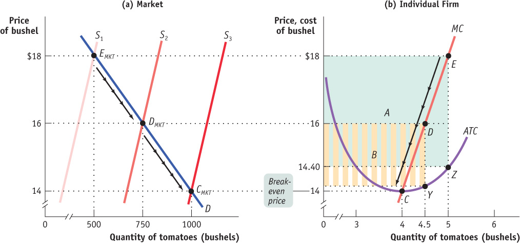
In the long run, these profits will induce new producers to enter the industry, shifting the short-
Although diminished, the profit of existing firms at DMKT means that entry will continue and the number of firms will continue to rise. If the number of producers rises to 250, the short-
A market is in long-run market equilibrium when the quantity supplied equals the quantity demanded, given that sufficient time has elapsed for entry into and exit from the industry to occur.
Like EMKT and DMKT, CMKT is a short-
To explore further the significance of the difference between short-
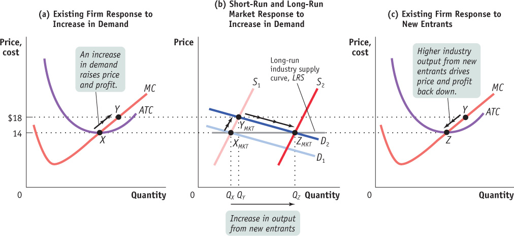
In panel (b) of Figure 12-7, D1 is the initial demand curve and S1 is the initial short-
Now suppose that the demand curve shifts out for some reason to D2. As shown in panel (b), in the short run, industry output moves along the short-
But we know that YMKT is not a long-
The effect of entry on an existing firm is illustrated in panel (c), in the movement from Y to Z along the firm’s individual supply curve. The firm reduces its output in response to the fall in the market price, ultimately arriving back at its original output quantity, corresponding to the minimum of its average total cost curve. In fact, every firm that is now in the industry—
The long-run industry supply curve shows how the quantity supplied responds to the price once producers have had time to enter or exit the industry.
The line LRS that passes through XMKT and ZMKT in panel (b) is the long-run industry supply curve. It shows how the quantity supplied by an industry responds to the price given that producers have had time to enter or exit the industry.
In this particular case, the long-
In other industries, however, even the long-
It is possible for the long-
Regardless of whether the long-
The distinction between the short-
The Cost of Production and Efficiency in Long-Run Equilibrium
Our analysis leads us to three conclusions about the cost of production and efficiency in the long-run equilibrium of a perfectly competitive industry. These results will be important in our discussion in Chapter 13 of how monopoly gives rise to inefficiency.
First, in a perfectly competitive industry in equilibrium, the value of marginal cost is the same for all firms. That’s because all firms produce the quantity of output at which marginal cost equals the market price, and as price-takers supplying a standardized product, they all face the same market price.
Second, in a perfectly competitive industry with free entry and exit, each firm will have zero economic profit in long-run equilibrium. Each firm produces the quantity of output that minimizes its average total cost—corresponding to point Z in panel (c) of Figure 12-7. So the total cost of production of the industry’s output is minimized in a perfectly competitive industry. (The exception is an industry with increasing costs across the industry. Given a sufficiently high market price, early entrants make positive economic profits, but the last entrants do not. At the long-run equilibrium price, average costs are minimized for later entrants, but not necessarily for the early ones. For early entrants, average costs depend on how much their cost curves have shifted up since the later entrants arrived.)
The third and final conclusion is that the long-run market equilibrium of a perfectly competitive industry is efficient: no mutually beneficial transactions go unexploited. To understand this, we need to recall a fundamental requirement for efficiency from Chapter 4: all consumers who have a willingness to pay greater than or equal to sellers’ costs actually get the good. And we also learned that when a market is efficient (except under certain, well-defined conditions), the market price matches all consumers with a willingness to pay greater than or equal to the market price to all sellers who have a cost of producing the good less than or equal to the market price.
ECONOMIC PROFIT, AGAIN
Some readers may wonder why a firm would want to enter an industry if the market price is only slightly greater than the break-even price. Wouldn’t a firm prefer to go into another business that yields a higher profit?
The answer is that here, as always, when we calculate cost, we mean opportunity cost—that is, cost that includes the return a firm could get by using its resources elsewhere. And so the profit that we calculate is economic profit; if the market price is above the break-even level, no matter how slightly, the firm can earn more in this industry than they could elsewhere.
So in the long-run equilibrium of a perfectly competitive industry, production is efficient: costs are minimized and no resources are wasted. In addition, the allocation of goods to consumers is efficient: every consumer willing to pay the cost of producing a unit of the good gets it. Indeed, no mutually beneficial transaction is left unexploited. Moreover, this condition tends to persist over time as the environment changes: the force of competition makes producers responsive to changes in consumers’ desires and to changes in technology.
BALEING IN, BAILING OUT
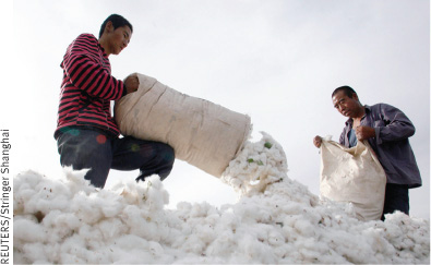
“King Cotton is back,” proclaimed a 2010 article in the Los Angeles Times, describing a cotton boom that had “turned great swaths of Central California a snowy white during harvest season.” Cotton prices were soaring: they more than tripled between early 2010 and early 2011. And farmers responded by planting more cotton.
What was behind the price rise? As we learned in Chapter 3, it was partly caused by temporary factors, notably severe floods in Pakistan that destroyed much of that nation’s cotton crop. But there was also a big rise in demand, especially from China, whose burgeoning textile and clothing industries demanded ever more raw cotton to weave into cloth. And all indications were that higher demand was here to stay.
So is cotton farming going to be a highly profitable business from now on? The answer is no, because when an industry becomes highly profitable, it draws in new producers, and that brings prices down. And the cotton industry was following the standard script.
For it wasn’t just the Central Valley of California that had turned “snowy white.” Farmers around the world were moving into cotton growing. “This summer, cotton will stretch from Queensland through northern NSW [New South Wales] all the way down to the Murrumbidgee valley in southern NSW,” declared an Australian report.
And by the summer of 2011 the entry of all these new producers was already having an effect. By the end of July, cotton prices were down 35% from their peak in early 2011. This still left prices high by historical standards, leaving plenty of incentive to expand production. But it was already clear that the cotton boom would eventually reach its limit—and that at some point in the not-too-distant future some of the farmers who had rushed into the industry would leave it again.

Quick Review
The industry supply curve corresponds to the supply curve of earlier chapters. In the short run, the time period over which the number of producers is fixed, the short-run market equilibrium is given by the intersection of the short-run industry supply curve and the demand curve. In the long run, the time period over which producers can enter or exit the industry, the long-run market equilibrium is given by the intersection of the long-run industry supply curve and the demand curve. In the long-run market equilibrium, no producer has an incentive to enter or exit the industry.
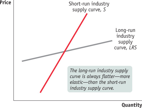
The long-run industry supply curve is often horizontal, although it may slope upward when a necessary input is in limited supply. It is always more elastic than the short-run industry supply curve.
In the long-run market equilibrium of a perfectly competitive industry, each firm produces at the same marginal cost, which is equal to the market price, and the total cost of production of the industry’s output is minimized. It is also efficient.
Check Your Understanding 12-3
CHECK YOUR UNDERSTANDING 12-3
Question 12.4
Which of the following events will induce firms to enter an industry? Which will induce firms to exit? When will entry or exit cease? Explain your answer.
A technological advance lowers the fixed cost of production of every firm in the industry.
The wages paid to workers in the industry go up for an extended period of time.
A permanent change in consumer tastes increases demand for the good.
The price of a key input rises due to a long-term shortage of that input.
A fall in the fixed cost of production generates a fall in the average total cost of production and, in the short run, an increase in each firm’s profit at the current output level. So in the long run new firms will enter the industry. The increase in supply drives down price and profits. Once profits are driven back to zero, entry will cease.
Click the figure to see a larger image
An increase in wages generates an increase in the average variable and the average total cost of production at every output level. In the short run, firms incur losses at the current output level, and so in the long run some firms will exit the industry. (If the average variable cost rises sufficiently, some firms may even shut down in the short run.) As firms exit, supply decreases, price rises, and losses are reduced. Exit will cease once losses return to zero.
Price will rise as a result of the increased demand, leading to a short-run increase in profits at the current output level. In the long run, firms will enter the industry, generating an increase in supply, a fall in price, and a fall in profits. Once profits are driven back to zero, entry will cease.
The shortage of a key input causes that input’s price to increase, resulting in an increase in average variable and average total costs for producers. Firms incur losses in the short run, and some firms will exit the industry in the long run. The fall in supply generates an increase in price and decreased losses. Exit will cease when losses have returned to zero.
Question 12.5
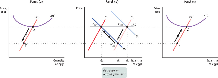
Assume that the egg industry is perfectly competitive and is in long-run equilibrium with a perfectly elastic long-run industry supply curve. Health concerns about cholesterol then lead to a decrease in demand. Construct a figure similar to Figure 12-7, showing the short-run behaviour of the industry and how long-run equilibrium is re-established.
In Figure 12-7, point XMKT in panel (b), the intersection of S1 and D1, represents the long-run industry equilibrium before the change in consumer tastes. When tastes change, demand falls and the industry moves in the short run to point YMKT in panel (b), at the intersection of the new demand curve D2 and S1, the short-run supply curve representing the same number of egg producers as in the original equilibrium at point XMKT. As the market price falls, an individual firm reacts by producing less—as shown in panel (a)—as long as the market price remains above the minimum average variable cost. If market price falls below minimum average variable cost, the firm would shut down immediately. At point YMKT the price of eggs is below minimum average total cost, creating losses for producers. This leads some firms to exit, which shifts the short-run industry supply curve leftward to S2. A new long-run equilibrium is established at point ZMKT. As this occurs, the market price rises again, and, as shown in panel (c), each remaining producer reacts by increasing output (here, from point Y to point Z). All remaining producers again make zero profits. The decrease in the quantity of eggs supplied in the industry comes entirely from the exit of some producers from the industry. The long-run industry supply curve is the curve labelled LRS in panel (b).
In Store and Online

Recently in Moncton, New Brunswick, Tri Trang walked into a Future Shop and found the perfect gift for his girlfriend, a $179.99 Garmin GPS system. A year earlier, he would have bought the item right away. Instead, he whipped out his Android phone; using an app that scans bar codes to instantly compare Future Shop’s price to those of other retailers, he found the same item on Amazon.ca for $134.98, with no shipping charges. Trang proceeded to buy it from Amazon, right there on the spot.
It doesn’t stop there. TheFind, the most popular price comparison site in the United States, will also provide a map to the store with the best price, identify coupon codes and shipping deals, and supply other tools to help users organize their purchases. “Terror” is the word that has been used to describe the reaction of brick-and-mortar retailers.
Before the advent of online price comparisons and smartphones, a retailer could lure customers into its store with enticing specials, and reasonably expect them to buy other, more profitable things, too—with some prompting from salespeople. But those days are disappearing. A recent study by the consulting firm Accenture found that 30% of Canadians use their mobile devices to assist their in-store shopping. According to a survey by GroupM Next, if the in-store and online price difference is close, shoppers will buy the product immediately in-store. But if the price difference is more than $15, most customers simply buy online instead.
Not surprisingly, use of apps like ShopSavvy, RedLaser (from eBay), or Price Check by Amazon (only available in the United States at the time of writing) has increased at an extremely fast clip. In the past few years e-commerce sales have risen by 20% or more per year. It is estimated that Cyber Monday in 2013 was the largest e-commerce day in history, and sales from mobile devices were responsible for between 20 and 25% of all e-commerce sales that day. Retailers are expecting even more shoppers to use their phones to make purchases in the coming years. The Canadian e-commerce market is expected to grow faster than the U.S. market, helping to bring it closer to the traditional ten-to-one U.S.-to-Canada ratio.
According to e-commerce experts, retailers have begun to alter their selling strategies in response. One strategy involves stocking products that manufacturers have slightly modified for the retailer, which allows the retailer to be their exclusive seller. Future Shop and Best Buy have closed stores, switched to smaller outlets, and rented space within their stores for in-store Microsoft mini stores and Sony kiosks. They have even partnered with affiliates to use Futureshop.ca and BestBuy.ca to sell products that they have not traditionally marketed: jewellery, luggage, furniture, children’s car seats, and home decor items like paints. In addition, some retailers, when confronted by an in-store customer wielding a lower price on a mobile device, will lower their price to avoid losing the sale (although other stores have responded by asking customers with price comparison apps to leave).
Retailers are clearly frightened. As one analyst said, “Only a couple of retailers can play the lowest-price game. This is going to accelerate the demise of retailers who do not have either competitive pricing or stand-out store experience.”
QUESTIONS FOR THOUGHT
Question 12.6
From the evidence in the case, what can you infer about whether or not the retail market for electronics satisfied the conditions for perfect competition before the advent of mobile-device comparison shopping? What was the most important impediment to competition?
Question 12.7
What effect will the introduction of price-comparison apps have on competition in the retail market for electronics? On the profitability of brick-and-mortar retailers like Future Shop? What, on average, will be the effect on the consumer surplus of purchasers of these items?
Question 12.8
Why are some retailers responding by having manufacturers make exclusive versions of products for them? Is this trend likely to increase or diminish?