16.2 Policies Toward Pollution
Before 1970, there were no rules governing the amount of sulphur dioxide power plants in North America could emit—
In this section we’ll look at the policies governments use to deal with pollution and at how economic analysis has been used to improve those policies.
Environmental Standards
The most serious external costs in the modern world are surely those associated with actions that damage the environment—
Environmental standards are rules that protect the environment by specifying actions by producers and consumers.
How does a country protect its environment? At present the main policy tools are environmental standards, rules that protect the environment by specifying actions by producers and consumers. A familiar example is the law that requires almost all vehicles to have catalytic converters, which reduce the emission of chemicals that can cause smog and lead to health problems. Other rules require communities to treat their sewage or factories to avoid or limit certain kinds of pollution, and so on.
Environmental standards came into widespread use in the 1960s and 1970s, and they have had considerable success in reducing pollution. For example, since the U.S. Clean Air Act in 1970, overall emission of pollutants into the air has fallen by more than a third, even though the U.S. population has grown by a third and the size of its economy has more than doubled. Even in Los Angeles, still famous for its smog, the air has improved dramatically: ozone levels in the South Coast Air Basin exceeded U.S. federal standards on 194 days in 1976; in 2010, on only 7 days. Air pollution levels in Hamilton, Ontario, another city with a long history of smog, have also been trending downward since the mid-
Despite these successes, economists believe that when regulators can control a polluter’s emissions directly, there are more efficient ways than environmental standards to deal with pollution. By using methods grounded in economic analysis, society can achieve a cleaner environment at lower cost. Most current environmental standards are inflexible and don’t allow reductions in pollution to be achieved at minimum cost. For example, two power plants—
How does economic theory suggest that pollution should be directly controlled? There are actually two approaches: taxes and tradable permits. As we’ll see, either approach can achieve the efficient outcome at the minimum feasible cost.
Emissions Taxes
An emissions tax is a tax that depends on the amount of pollution a firm produces.
One way to deal with pollution directly is to charge polluters an emissions tax. Emissions taxes are taxes that depend on the amount of pollution a firm produces. For example, power plants might be charged $200 for every tonne of sulphur dioxide they emit.
Look again at Figure 16-2, which shows that the socially optimal quantity of pollution is QOPT. At that quantity of pollution, the marginal social benefit and marginal social cost of an additional tonne of emissions are equal at $200. But in the absence of government intervention, power companies have no incentive to limit pollution to the socially optimal quantity, QOPT; instead, they will push pollution up to the quantity QMKT, at which marginal social benefit is zero.
It’s now easy to see how an emissions tax can solve the problem. If power companies are required to pay a tax of $200 per tonne of emissions, they now face a marginal cost of $200 per tonne and have an incentive to reduce emissions to QOPT, the socially optimal quantity. This illustrates a general result: an emissions tax equal to the marginal social cost at the socially optimal quantity of pollution induces polluters to internalize the externality—
ECONOMIC GROWTH AND GREENHOUSE GASES IN SIX COUNTRIES
At first glance, a comparison of the per capita greenhouse gas emissions of various countries, shown in panel (a) of this graph, suggests that Australia, Canada, and the United States are the worst offenders. The average Canadian is responsible for 22.9 tonnes of greenhouse gas emissions (measured in CO2 equivalents)—the pollution that causes global warming—
Such a conclusion, however, ignores an important factor in determining the level of a country’s greenhouse gas emissions: its gross domestic product, or GDP—
A more meaningful way to compare pollution across countries is to measure emissions per $1 million of a country’s GDP, as shown in panel (b). On this basis, the United States, Canada, India, and Australia are now “green” countries, but China and Uzbekistan are not. What explains the reversal once GDP is accounted for? The answer: both economics and government behaviour.
First, there is the issue of economics. Countries that are poor and have begun to industrialize, such as Uzbekistan, often view money spent to reduce pollution as better spent on other things. From their perspective, they are still too poor to afford as clean an environment as wealthy advanced countries. They claim that to impose a wealthy country’s environmental standards on them would jeopardize their economic growth.
Second, there is the issue of government behaviour—
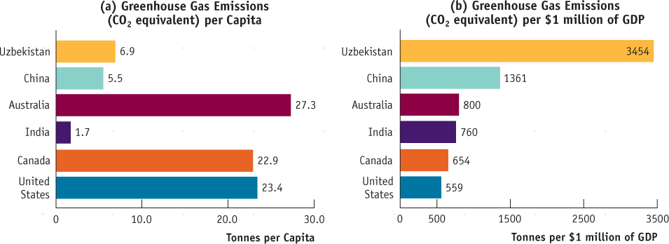
Source: World Resources Institute.
Why is an emissions tax an efficient way (that is, a cost-
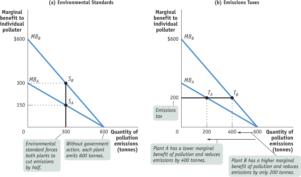
In the absence of government action, we know that polluters will pollute until the marginal social benefit of an additional unit of emissions is equal to zero. Recall that the marginal social benefit of pollution is the cost savings, at the margin, to polluters of an additional unit of pollution. As a result, without government intervention each plant will pollute until its own marginal benefit of pollution is equal to zero. This corresponds to an emissions quantity of 600 tonnes each for plants A and B—
Now suppose that the government decides that overall pollution from this industry should be cut in half, from 1200 tonnes to 600 tonnes. Panel (a) of Figure 16-4 shows how this might be achieved with an environmental standard that requires each plant to cut its emissions in half, from 600 to 300 tonnes. The standard has the desired effect of reducing overall emissions from 1200 to 600 tonnes but accomplishes it in an inefficient way. As you can see from panel (a), the environmental standard leads plant A to produce at point SA, where its marginal benefit of pollution is $150, but plant B is now producing at point SB, where its marginal benefit of pollution is twice as high, $300.
This difference in marginal benefits between the two plants tells us that the same quantity of pollution can be achieved at lower total cost by allowing plant B to pollute more than 300 tonnes but inducing plant A to pollute less. In fact, the efficient way to reduce pollution is to ensure that at the industry-
We can see from panel (b) how an emissions tax achieves exactly that result. Suppose both plant A and plant B pay an emissions tax of $200 per tonne, so that the marginal cost of an additional tonne of emissions to each plant is now $200 rather than zero. As a result, plant A produces at TA and plant B produces at TB. So plant A reduces its pollution more than it would under an inflexible environmental standard, cutting its emissions from 600 to 200 tonnes; meanwhile, plant B reduces its pollution less, going from 600 to 400 tonnes. In the end, total pollution—
Taxes designed to reduce external costs are known as Pigouvian taxes.
The term emissions tax may convey the misleading impression that taxes are a solution to only one kind of external cost, pollution. In fact, taxes can be used to discourage any activity that generates negative externalities, such as driving during rush hour or operating a noisy bar in a residential area. In general, taxes designed to reduce external costs are known as Pigouvian taxes, after the economist A. C. Pigou, who emphasized their usefulness in his classic 1920 book, The Economics of Welfare. In our example, the optimal Pigouvian tax is $200; as you can see from Figure 16-2, this corresponds to the marginal social cost of pollution at the socially optimal output quantity, QOPT.
Are there any problems with emissions taxes? The main concern is that in practice government officials usually aren’t sure how high the tax should be set. If they set the tax too low, there will be too little improvement in the environment; if they set it too high, emissions will be reduced by more than is efficient. This uncertainty cannot be eliminated, but the nature of the risks can be changed by using an alternative strategy, issuing tradable emissions permits.
The Pigouvian Tax in the Competitive Market
Rather than levy a tax directly on pollution, it is possible to impose the tax on the production of the good whose production or consumption results in the creation of the pollution. Figure 16-5 below revisits the competitive market for electricity with an optimal Pigouvian tax.
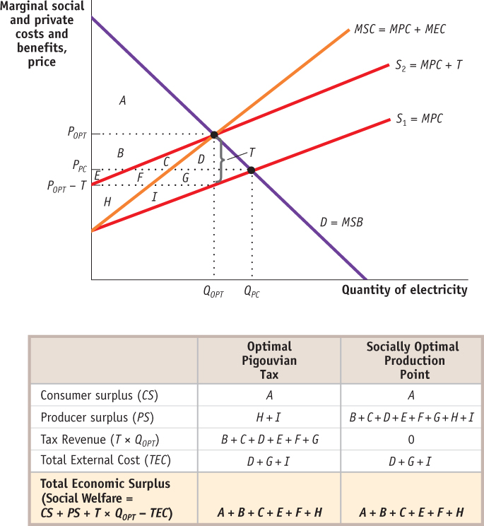
Suppose an excise tax is imposed on electricity producers. This per-
After the tax is applied, the consumer surplus is equal to area A, the producer surplus is equal to the sum of areas H and I, while the government tax revenue is the rectangle made up of B, C, D, E, F, and G. Since the total external cost is the area between the MSC and supply curves it equals the sum of the areas D, G, and I. So with the tax, the total economic surplus is equal to the sum of the areas A, B, C, E, F, and H. The calculations in the table in Figure 16-5 show that this outcome is socially efficient. By charging a per-
Tradable Emissions Permits
Tradable emissions permits are licences to emit limited quantities of pollutants that can be bought and sold by polluters.
Tradable emissions permits are licences to emit limited quantities of pollutants that can be bought and sold by polluters. They are usually issued to polluting firms according to some formula reflecting their history. For example, each power plant might be issued permits equal to 50% of its emissions before the system went into effect. The more important point, however, is that these permits are tradable. Firms with differing costs of reducing pollution can now engage in mutually beneficial transactions: those that find it easier to reduce pollution will sell some of their permits to those that find it more difficult.
In other words, firms will use transactions in permits to reallocate pollution reduction among themselves, so that in the end those with the lowest cost will reduce their pollution the most, and those with the highest cost will reduce their pollution the least. Assume that the government issues 300 licences each to plant A and plant B, where one licence allows the emission of one tonne of pollution. Under a system of tradable emissions permits, plant A will find it profitable to sell 100 of its 300 government-
Just like emissions taxes, tradable permits provide polluters with an incentive to take the marginal social cost of pollution into account. To see why, suppose that the market price of a permit to emit one tonne of sulphur dioxide is $200. Then every plant has an incentive to limit its emissions of sulphur dioxide to the point where its marginal benefit of emitting another tonne of pollution is $200. This is obvious for plants that buy rights to pollute: if a plant must pay $200 for the right to emit an additional tonne of sulphur dioxide, it faces the same incentives as a plant facing an emissions tax of $200 per tonne.
But it’s equally true for plants that have more permits than they plan to use: by not emitting a tonne of sulphur dioxide, a plant frees up a permit that it can sell for $200, so the opportunity cost of a tonne of emissions to the plant’s owner is $200.
In short, tradable emissions permits have the same cost-
It’s important to realize that emissions taxes and tradable permits do more than induce polluting industries to reduce their output. Unlike rigid environmental standards, emissions taxes and tradable permits provide incentives to create and use technology that emits less pollution—
The main problem with tradable emissions permits is the flip-
Lacking any significant new federal action, in 2008 British Columbia, Manitoba, Ontario, and Quebec, committed to joining the Western Climate Initiative: a tradable permits market in Canada and the United States that seeks to reduce greenhouse gas emissions and the negative externalities they create. After first relying on environmental standards, the U.S. government has turned to a system of tradable permits to control acid rain. And in 2005 the European Union created the largest emissions-
Emissions Taxes Versus Tradable Emissions Permits
It turns out that a tax on emissions of greenhouse gases, like the carbon tax in British Columbia, can have the exact same outcome as a system of tradable emissions permit. Figure 16-6 below helps to convey this point.
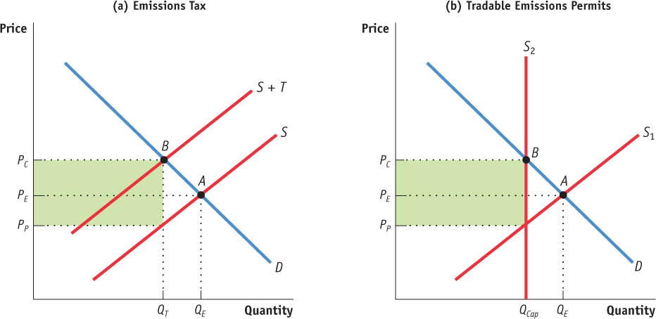
Using a system of tradable emissions permits makes the supply curve perfectly vertical at the government imposed maximum level of output, as shown in panel (b). This reduces the quantity of the product exchanged and raises the price that consumers pay. If the permits are free, the green-shaded area represents profits captured by firms. If permits are sold by the government, this area represents the revenue for the government.
Suppose we have a product whose production results in the emission of greenhouse gases. Panel (a) of Figure 16-6 shows the impact of a tax on greenhouse gas emissions that is levied on the suppliers of this product. Imposing an excise tax, T, per unit shifts the supply curve up to (S + T) and moves the market equilibrium from A to B. In the new equilibrium, the quantity exchanged has declined (from QE to QT), the price paid by consumers has increased (from PE to PC), and the price received by producers will decline (from PE to PP, where PP = PC – T). The tax revenue is equal to the area shaded in green in Figure 16-6 (Tax revenue = T × QT).
Now what if the government decides to impose a system of tradable emissions permits instead? Such a system is described in panel (b) of Figure 16-6: the government creates a volume limit or “cap” on the total quantity of the product that can be supplied. In effect, this makes the supply curve perfectly vertical and shifts it to the left to the new (lower) government imposed upper bound on production. This new supply curve is labelled S2 in the diagram. In the new equilibrium at B, the quantity exchanged has declined (from QE to QCap) and the price paid by consumers has increased (from PE to PC). If the government issues permits freely, the firms receiving them capture the shaded area as profit since the price earned by firms (PC) exceeds their cost of production (PP). Alternatively, if the government sells the permits, then the green-shaded area is equal to the governments permit revenue and firms earn zero profit.
The lesson is simple. It does not matter whether the government uses an emissions tax or a tradable emissions system; if properly designed both can result in exactly the same outcome for society.
CAP AND TRADE

Unlike the Western Climate Initiative, the tradable emissions permit systems for both acid rain in the United States and greenhouse gases in the European Union are examples of cap and trade systems: the government sets a cap (a maximum amount of pollutant that can be emitted), issues tradable emissions permits, and enforces a yearly rule that a polluter must hold a number of permits equal to the amount of pollutant emitted. The goal is to set the cap low enough to generate environmental benefits, while giving polluters flexibility in meeting environmental standards and motivating them to adopt new technologies that will lower the cost of reducing pollution.
Starting in the 1980s, the federal government used a cap and trade system to help phase out the consumption of CFCs, methyl bromide, and HCFCs, all of which depleted the ozone layer. But since this successful cap and trade experiment, the federal government has stayed away from introducing either a larger cap and trade system for greenhouse gases or a carbon tax. At the provincial level, Alberta and Ontario have each set up cap and trade systems for nitrogen oxide and sulphur dioxide emitted by large electricity generators. In 2013, Quebec started a cap and trade system for industrial emissions of greenhouse gases. Quebec intends to merge this market with the Western Climate Initiative.
In 1994 the United States began a cap and trade system for the sulphur dioxide emissions that cause acid rain. Thanks to the system, air pollutants decreased by more than 40% from 1990 to 2008, and 2010 acid rain levels dropped to approximately 50% of their 1980 levels. Economists who have analyzed the sulphur dioxide cap and trade system point to another reason for its success: it would have been 80% more expensive to reduce emissions by this much using a non-market-based regulatory policy.
The EU cap and trade scheme, covering all 28 member nations of the European Union, is the world’s only mandatory trading scheme for greenhouse gases. It is scheduled to achieve a 21% reduction in greenhouse gases by 2020 compared to 2005 levels.
Other countries, like Australia and New Zealand, have adopted less comprehensive trading schemes for greenhouse gases. According to the World Bank, the worldwide market for greenhouse gases—also called carbon trading—has grown rapidly, from $11 billion in permits traded in 2005 to $142 billion in 2010. In New Zealand, famous for its sheep and lamb industry, farmers are busy converting grazing land into forests so that they can sell permits beginning in 2015, when companies will be required to pay for their emissions.
Despite all this good news, however, cap and trade systems are not silver bullets for the world’s pollution problems. Although they are appropriate for pollution that’s geographically dispersed, like sulphur dioxide and greenhouse gases, they don’t work for pollution that’s localized, like mercury or lead contamination. In addition, the amount of overall reduction in pollution depends on the level of the cap. Under industry pressure, regulators run the risk of issuing too many permits, effectively eliminating the cap. Finally, there must be vigilant monitoring of compliance if the system is to work. Without oversight of how much a polluter is actually emitting, there is no way to know for sure that the rules are being followed.

Quick Review
Governments often limit pollution with environmental standards. Generally, such standards are an inefficient way to reduce pollution because they are inflexible.
When the quantity of pollution emitted can be directly observed and controlled, environmental goals can be achieved efficiently in two ways: emissions taxes and tradable emissions permits. These methods are efficient because they are flexible, allocating more pollution reduction to those who can do it more cheaply. They also motivate polluters to adopt new pollution-reducing technology.
An emissions tax and an excise tax on a good resulting in pollution are forms of Pigouvian tax. The optimal Pigouvian tax is equal to the marginal social cost of pollution at the socially optimal quantity of pollution.
Check Your Understanding 16-2
CHECK YOUR UNDERSTANDING 16-2
Question 16.3
Some opponents of tradable emissions permits object to them on the grounds that polluters that sell their permits benefit monetarily from their contribution to polluting the environment. Assess this argument.
This is a misguided argument. Allowing polluters to sell emissions permits makes polluters face a cost of polluting: the opportunity cost of the permit. If a polluter chooses not to reduce its emissions, it cannot sell its emissions permits. As a result, it forgoes the opportunity of making money from the sale of the permits. So despite the fact that the polluter receives a monetary benefit from selling the permits, the scheme has the desired effect: to make polluters internalize the externality of their actions.
Question 16.4
Explain the following.
Why an emissions tax smaller than or greater than the marginal social cost at QOPT leads to a smaller total surplus compared to the total surplus generated if the emissions tax had been set optimally
Why a system of tradable emissions permits that sets the total quantity of allowable pollution higher or lower than QOPT leads to a smaller total surplus compared to the total surplus generated if the number of permits had been set optimally
If the emissions tax is smaller than the marginal social cost at QOPT, a polluter will face a marginal cost of polluting (equal to the amount of the tax) that is less than the marginal social cost at the socially optimal quantity of pollution. Since a polluter will produce emissions up to the point where the marginal social benefit is equal to its marginal cost, the resulting amount of pollution will be larger than the socially optimal quantity. As a result, there is inefficiency: if the amount of pollution is larger than the socially optimal quantity, the marginal social cost exceeds the marginal social benefit, and society could gain from a reduction in emissions levels.
If the emissions tax is greater than the marginal social cost at QOPT, a polluter will face a marginal cost of polluting (equal to the amount of the tax) that is greater than the marginal social cost at the socially optimal quantity of pollution. This will lead the polluter to reduce emissions below the socially optimal quantity. This also is inefficient: whenever the marginal social benefit is greater than the marginal social cost, society could benefit from an increase in emissions levels.
If the total amount of allowable pollution is set too high, the supply of emissions permits will be high and so the equilibrium price at which permits trade will be low. That is, polluters will face a marginal cost of polluting (the price of a permit) that is “too low”—lower than the marginal social cost at the socially optimal quantity of pollution. As a result, pollution will be greater than the socially optimal quantity. This is inefficient.
If the total level of allowable pollution is set too low, the supply of emissions permits will be low and so the equilibrium price at which permits trade will be high. That is, polluters will face a marginal cost of polluting (the price of a permit) that is “too high”—higher than the marginal social cost at the socially optimal quantity of pollution. As a result, pollution will be lower than the socially optimal quantity. This also is inefficient.