20.1 The Economics of Risk Aversion
In general, people don’t like risk and are willing to pay a price to avoid it. Just ask the global insurance industry, which collects more than US$4.6 trillion in premiums every year, including more than $100 billion in Canada alone. But what exactly is risk? And why don’t most people like it? To answer these questions, we need to look briefly at the concept of expected value and the meaning of uncertainty. Then we can turn to why people dislike risk.
Expectations and Uncertainty
The Lee family doesn’t know how big its medical bills will be next year. If all goes well, it won’t have any medical expenses at all. Let’s assume that there’s a 50% chance of that happening. But if family members require out-
A random variable is a variable with an uncertain future value.
In this example—
The expected value of a random variable is the weighted average of all possible values, where the weights on each possible value correspond to the probability of that value occurring.
To derive the general formula for the expected value of a random variable, we imagine that there are a number of different states of the world, possible future events. Each state is associated with a different realized value—
A state of the world is a possible future event.
In the case of the Lee family, there are only two possible states of the world, each with a probability of 0.5.
Notice, however, that the Lee family doesn’t actually expect to pay $5000 in medical bills next year. That’s because in this example there is no state of the world in which the family pays exactly $5000. Either the family pays nothing, or it pays $10 000. So the Lees face considerable uncertainty about their future medical expenses.
But what if the Lee family can buy supplemental health insurance that will cover any medical expenses they face that are not covered by a government health insurance plan, whatever they turn out to be? Suppose, in particular, that the family can pay $5000 up front in return for full coverage of whatever medical expenses actually arise during the coming year. Then the Lees’s future medical expenses are no longer uncertain for them: in return for $5000—an amount equal to the expected value of the medical expenses—
Risk is uncertainty about future outcomes. When the uncertainty is about monetary outcomes, it becomes financial risk.
Yes, it would—
The Logic of Risk Aversion
To understand how diminishing marginal utility gives rise to risk aversion, we need to look not only at the Lees’s medical costs but also at how those costs affect the income the family has left after medical expenses. Let’s assume the family knows that it will have an income of $30 000 next year. If the family has no medical expenses, it will be left with all of that income. If its medical expenses are $10 000, its income after medical expenses will be only $20 000. Since we have assumed that there is an equal chance of these two outcomes, the expected value of the Lees’s income after medical expenses is (0.5 × $30 000) + (0.5 × $20 000) = $25 000. At times we will simply refer to this as expected income.
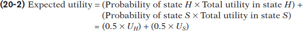
Expected utility is the expected value of an individual’s total utility given uncertainty about future outcomes.
But as we’ll now see, if the family’s utility function has the shape typical of most families’, its expected utility—the expected value of its total utility given uncertainty about future outcomes—
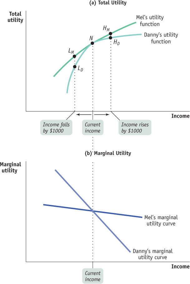
To see why, we need to look at how total utility depends on income. Panel (a) of Figure 20-1 shows a hypothetical utility function for the Lee family, where total utility depends on income—
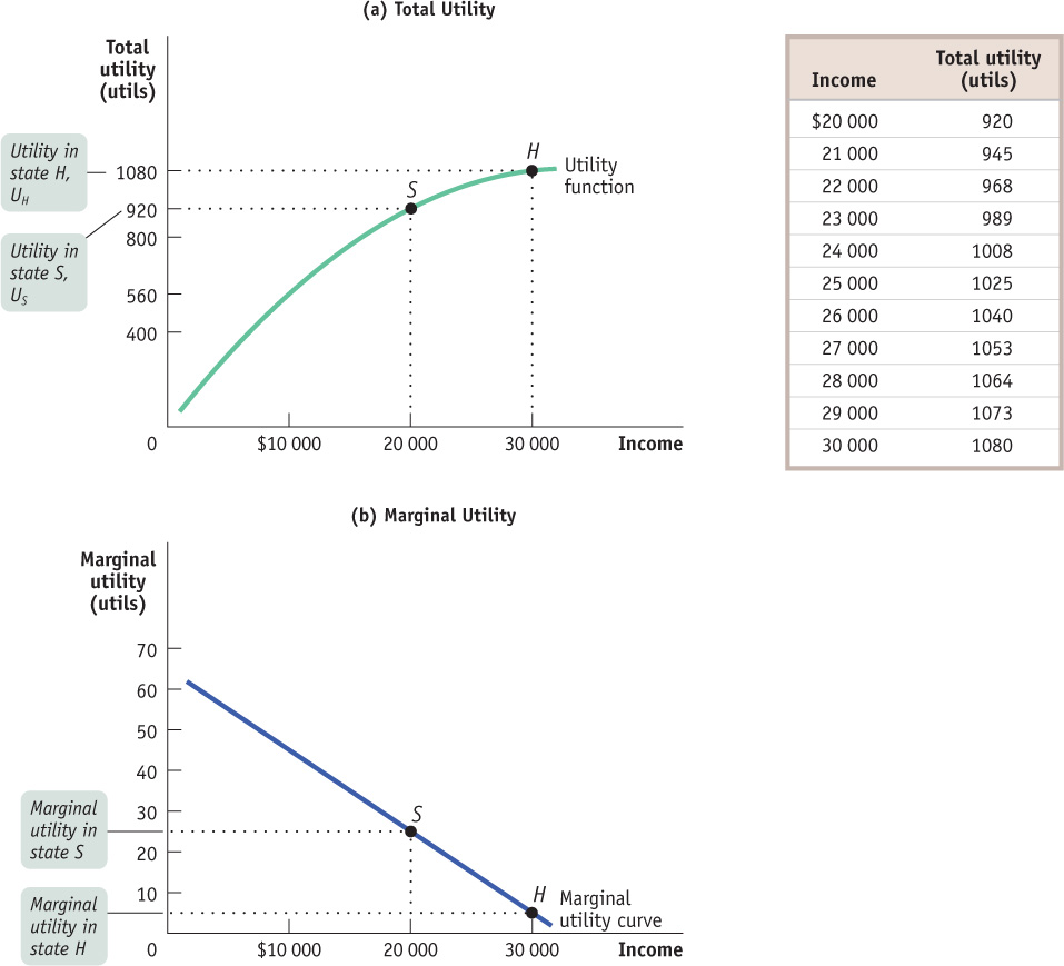
In Chapter 10 we applied the principle of diminishing marginal utility to individual goods and services: each successive unit of a good or service that a consumer purchases adds less to his or her total utility. The same principle applies to income used for consumption: each successive dollar of income adds less to total utility than the previous dollar. Panel (b) shows how marginal utility varies with income, confirming that marginal utility of income falls as income rises. As we’ll see in a moment, diminishing marginal utility is the key to understanding the desire of individuals to reduce risk.
To analyze how a person’s utility is affected by risk, economists start from the assumption that individuals facing uncertainty maximize their expected utility. We can use the data in Figure 20-1 to calculate the Lee family’s expected utility. We’ll first do the calculation assuming that the Lees have no supplemental insurance, and then we’ll recalculate it assuming that they have purchased supplemental insurance.
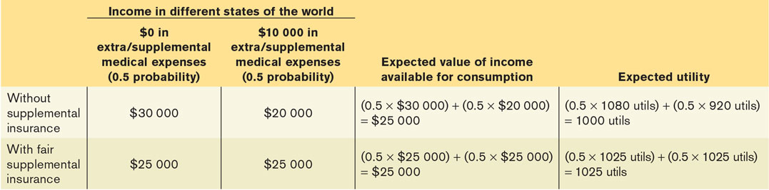
Without supplemental insurance, if the Lees are lucky and don’t incur any medical expenses, they will have an income of $30 000, generating total utility of 1080 utils. But if they have no supplemental insurance and are unlucky, incurring $10 000 in medical expenses, they will have just $20 000 of their income to spend on consumption and total utility of only 920 utils. So without supplemental insurance, the family’s expected utility is (0.5 × 1080) + (0.5 × 920) = 1000 utils.
A premium is a payment to an insurance company in return for the insurance company’s promise to pay a claim in certain states of the world.
Now let’s suppose that an insurance company offers to pay whatever medical expenses the family incurs during the next year in return for a premium—a payment to the insurance company—
A fair insurance policy is an insurance policy for which the premium is equal to the expected value of the claim.
If the family purchases this fair insurance policy, the expected value of its income available for consumption is the same as it would be without insurance: $25 000—that is, $30 000 minus the $5000 premium. But the family’s risk has been eliminated: the family has an income available for consumption of $25 000 for sure, which means that it receives the utility level associated with an income of $25 000. Reading from the table in Figure 20-1, we see that this utility level is 1025 utils. Or to put it a slightly different way, their expected utility with supplemental insurance is 1 × 1025 = 1025 utils, because with supplemental insurance they will receive a utility of 1025 utils with a probability of 1. And this is higher than the level of expected utility without supplemental insurance—
The calculations for this example are summarized in Table 20-1. This example shows that the Lees, like most people in real life, are risk-averse: they will choose to reduce the risk they face when the cost of that reduction leaves the expected value of their income or wealth unchanged. So the Lees, like most people, will be willing to buy fair insurance. Similarly, being risk-
Risk-averse individuals will choose to reduce the risk they face when that reduction leaves the expected value of their income or wealth unchanged.
You might think that this result depends on the specific numbers we have chosen. In fact, however, the proposition that the purchase of a fair insurance policy increases expected utility depends on only one assumption: diminishing marginal utility. The reason is that with diminishing marginal utility, a dollar gained when income is low adds more to utility than a dollar gained when income is high. That is, having an additional dollar matters more when you are facing hard times than when you are facing good times. And as we will shortly see, a fair insurance policy is desirable because it transfers a dollar from high-
But first, let’s see how diminishing marginal utility leads to risk aversion by examining expected utility more closely. In the case of the Lee family, there are two states of the world; let’s call them H and S, for healthy and sick. In state H the family has no medical expenses; in state S it has $10 000 in medical expenses. Let’s use the symbols UH and US to represent the Lee family’s total utility in each state. Then the family’s expected utility is:
The fair insurance policy reduces the family’s income available for consumption in state H by $5000, but it increases it in state S by the same amount. As we’ve just seen, we can use the utility function to directly calculate the effects of these changes on expected utility. But as we have also seen in many other contexts, we gain more insight into individual choice by focusing on marginal utility.
To use marginal utility to analyze the effects of fair insurance, let’s imagine introducing the insurance a bit at a time, say in 5000 small steps. At each of these steps, we reduce income in state H by $1 and simultaneously increase income in state S by $1. At each of these steps, total utility in state H falls by the marginal utility of income in that state but total utility in state S rises by the marginal utility of income in that state.
Now look again at panel (b) of Figure 20-1, which shows how marginal utility varies with income. Point S shows marginal utility when the Lee family’s income is $20 000; point H shows marginal utility when income is $30 000. Clearly, marginal utility is higher when income after medical expenses is low. Because of diminishing marginal utility, an additional dollar of income adds more to total utility when the family has low income (point S) than when it has high income (point H).
This tells us that the gain in expected utility from increasing income in state S is larger than the loss in expected utility from reducing income in state H by the same amount. So at each step of the process of reducing risk, by transferring $1 of income from state H to state S, expected utility increases. This is the same as saying that the family is risk-
Almost everyone is risk-
THE PARADOX OF GAMBLING

If most people are risk-
After all, a casino doesn’t even offer gamblers a fair gamble: all the games in any gambling facility are designed so that, on average, the casino makes money. So why would anyone play their games?
You might argue that the gambling industry caters to the minority of people who are actually the opposite of risk-
So why do people gamble? Presumably because they enjoy the experience.
Also, gambling may be one of those areas where the assumption of ration-
A risk-neutral person is completely insensitive to risk.
Panel (a) of Figure 20-2 shows how each individual’s total utility would be affected by the change in income. Danny would gain very few utils from a rise in income, which moves him from N to HD, but lose a large number of utils from a fall in income, which moves him from N to LD. That is, he is highly risk-
Individuals differ in risk aversion for two main reasons: differences in preferences and differences in initial income or wealth.
Differences in preferences. Other things equal, people simply differ in how much their marginal utility is affected by their level of income. Someone whose marginal utility is relatively unresponsive to changes in income will be much less sensitive to risk. In contrast, someone whose marginal utility depends greatly on changes in income will be much more risk-
averse. Differences in initial income or wealth. The possible loss of $1000 makes a big difference to a family living below the poverty line; it makes very little difference to someone who earns $1 million a year. In general, people with high incomes or high wealth will be less risk-
averse.
Differences in risk aversion have an important consequence: they affect how much an individual is willing to pay to avoid risk.
BEFORE THE FACT VERSUS AFTER THE FACT
Why is an insurance policy different from a doughnut?
No, it’s not a riddle. Although the supply and demand for insurance behave like the supply and demand for any good or service, the payoff is very different. When you buy a doughnut, you know what you’re going to get; when you buy insurance, by definition you don’t know what you’re going to get. If you bought car insurance and then didn’t have an accident, you got nothing from the policy, except peace of mind, and might wish that you hadn’t bothered. But if you did have an accident, you probably would be glad that you bought insurance that covered the cost.
This means we have to be careful in assessing the rationality of insurance purchases (or, for that matter, any decision made in the face of uncertainty). After the fact—after the uncertainty has been resolved—
One highly successful Wall Street investor told us that he never looks back—
Paying to Avoid Risk
The risk-averse Lee family is clearly better off taking out a fair insurance policy—a policy that leaves their expected income unchanged but eliminates their risk. Unfortunately, real insurance policies are rarely fair: because insurance companies have to cover other costs, such as salaries for salespeople and actuaries, they charge more than they expect to pay in claims. Will the Lee family still want to purchase an “unfair” insurance policy—one for which the premium is larger than the expected claim?
It depends on the size of the premium. Look again at Table 20-1. We know that without supplemental insurance, expected utility is 1000 utils. Also, supplemental insurance costing $5000 raises expected utility to 1025 utils. If the premium were $6000, the Lees would be left with an income of $24 000, which, as you can see from Figure 20-1, would give them a total utility of 1008 utils—which is still higher than their expected utility if they had no supplemental insurance at all. So the Lees would be willing to buy supplemental insurance with a $6000 premium. But they wouldn’t be willing to pay $7000, which would reduce their income to $23 000 and their total utility to 989 utils.
This example shows that risk-averse individuals are willing to make deals that reduce their expected income but also reduce their risk: they are willing to pay a premium that exceeds their expected claim. The more risk-averse they are, the higher the premium they are willing to pay. That willingness to pay is what makes the insurance industry possible. In contrast, a risk-neutral person is unwilling to pay anything at all to reduce his or her risk.
WARRANTIES

Many expensive consumer goods—electronic devices, major appliances, cars—come with some form of warranty. Typically, the manufacturer guarantees to repair or replace the item if something goes wrong with it during some specified period after purchase—usually six months or one year.
Why do manufacturers offer warranties? Part of the answer is that warranties signal to consumers that the goods are of high quality. But mainly warranties are a form of consumer insurance. For many people, the cost of repairing or replacing an expensive item like a refrigerator—or, worse yet, a car—would be a serious burden. If they were obliged to come up with the cash, their consumption of other goods would be restricted; as a result, their marginal utility of income would be higher than if they didn’t have to pay for repairs.
So a warranty that covers the cost of repair or replacement increases the consumer’s expected utility, even if the cost of the warranty is greater than the expected future claim paid by the manufacturer.

Quick Review
The expected value of a random variable is the weighted average of all possible values, where the weight corresponds to the probability of a given value occurring.
Uncertainty about states of the world entails risk, or financial risk when there is an uncertain monetary outcome. When faced with uncertainty, consumers choose the option yielding the highest level of expected utility.
Most people are risk-averse: they would be willing to purchase a fair insurance policy in which the premium is equal to the expected value of the claim.
Risk aversion arises from diminishing marginal utility. Differences in preferences and in income or wealth lead to differences in risk aversion.
Depending on the size of the premium, a risk-averse person may be willing to purchase an “unfair” insurance policy with a premium larger than the expected claim. The greater your risk aversion, the greater the premium you are willing to pay. A risk-neutral person is unwilling to pay any premium to avoid risk.
Check Your Understanding 20-1
CHECK YOUR UNDERSTANDING 20-1
Question 20.1
Compare two families who own homes near the floodplain of the Red River in Manitoba. Which family is likely to be more risk-averse—(i) a family with income of $2 million per year or (ii) a family with income of $60 000 per year? Would either family be willing to buy an “unfair” insurance policy to cover losses to their Manitoba home?
The family with the lower income is likely to be more risk-averse. In general, higher income or wealth results in lower degrees of risk aversion, due to diminishing marginal utility. Both families may be willing to buy an “unfair” insurance policy. Most insurance policies are “unfair” in that the expected claim is less than the premium. The degree to which a family is willing to pay more than an expected claim for insurance depends on the family’s degree of risk aversion.
Question 20.2
Karma’s income next year is uncertain: there is a 60% probability she will make $22 000 and a 40% probability she will make $35 000. The accompanying table shows some income and utility levels for Karma.
What is Karma’s expected income? Her expected utility?
What certain income level, sometimes called the certainty equivalent, leaves her as well off as her uncertain income? What does this imply about Karma’s attitudes toward risk? Explain.
Would Karma be willing to pay some amount of money greater than zero for an insurance policy that guarantees her an income of $26 000? Explain.
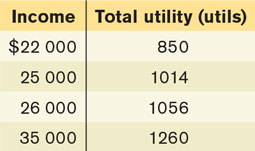
Karma’s expected income is the weighted average of all possible values of her income, weighted by the probabilities with which she earns each possible value of her income. Since she makes $22 000 with a probability of 0.6 and $35 000 with a probability of 0.4, her expected income is (0.6 × $22 000) + (0.4 × $35 000) = $13 200 + $14 000 = $27 200. Her expected utility is simply the expected value of the total utilities she will experience. Since with a probability of 0.6 she will experience a total utility of 850 utils (the utility to her from making $22 000), and with a probability of 0.4 she will experience a total utility of 1260 utils (the utility to her from making $35 000), her expected utility is (0.6 × 850 utils) + (0.4 × 1260 utils) = 510 utils + 504 utils = 1014 utils.
If Karma makes $25 000 for certain, she experiences a utility level of 1014 utils. From the answer to part (a), we know that this leaves her equally as well off as when she has a risky expected income of $27 200. Since Karma is indifferent between a risky expected income of $27 200 and a certain income of $25 000, you can conclude that she would prefer a certain income of $27 200 to a risky expected income of $27 200. That is, she would definitely be willing to reduce the risk she faces when this reduction in risk leaves her expected income unchanged. In other words, Karma is risk-averse.
Yes. Karma experiences a utility level of 1056 utils when she has a certain income of $26 000. This is higher than the expected utility level of 1014 utils generated by a risky expected income of $27 200. So Karma is willing to pay a premium to guarantee a certain income of $26 000.