6.4 The Price Elasticity of Supply
In the wake of a flu vaccine shortfall, attempts by vaccine distributors to drive up the price of vaccines would have been much less effective if the higher price had induced a large increase in the output of flu vaccines by other manufacturers. In fact, if a rise in price precipitated a significant increase in flu vaccine production, the price would be pushed back down. But that wouldn’t happen because, as we mentioned earlier, it is far too costly and technically difficult to produce more vaccine for the flu season in a short period of time. (In reality, the production of flu vaccine begins a year before distribution.)
This is another critical element in the ability of some flu vaccine distributors, like our hypothetical company Flunomics, to get significantly higher prices by restricting supply of their product: a low responsiveness in the quantity of output supplied to the higher price of flu vaccine by flu vaccine producers. To measure the response of producers to price changes, we need a measure parallel to the price elasticity of demand—
Measuring the Price Elasticity of Supply
The price elasticity of supply is a measure of the responsiveness of the quantity of a good supplied to the price of that good. It is the ratio of the percentage change in the quantity supplied to the percentage change in the price as we move along the supply curve.
The price elasticity of supply is defined the same way as the price elasticity of demand (although there is no minus sign to be eliminated here):

The only difference is that here we consider movements along the supply curve rather than movements along the demand curve.
Suppose that the price of tomatoes rises by 10%. If the quantity of tomatoes supplied also increases by 10% in response, the price elasticity of supply of tomatoes is 1 (10%/10%) and supply is unit-
As in the case of demand, the extreme values of the price elasticity of supply have a simple graphical representation. Panel (a) of Figure 6-6 shows the supply of cellphone frequencies, the portion of the radio spectrum that is suitable for sending and receiving cellphone signals. Governments own the right to sell the use of this part of the radio spectrum to cellphone operators inside their borders. But governments can’t increase or decrease the number of cellphone frequencies that they have to offer—
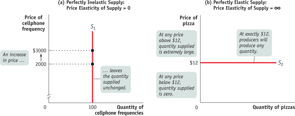
There is perfectly inelastic supply when the price elasticity of supply is zero, so that changes in the price of the good have no effect on the quantity supplied. A perfectly inelastic supply curve is a vertical line.
So the supply curve for cellphone frequencies is a vertical line, which we have assumed is set at the quantity of 100 frequencies. As you move up and down that curve, the change in the quantity supplied by the government is zero, whatever the change in price. So panel (a) illustrates a case in which the price elasticity of supply is zero. This is a case of perfectly inelastic supply.
Panel (b) shows the supply curve for pizza. We suppose that it costs $12 to produce a pizza, including all opportunity costs. At any price below $12, it would be unprofitable to produce pizza and all the pizza parlours in Canada would go out of business. Alternatively, there are many producers who could operate pizza parlours if they were profitable. The ingredients—
There is perfectly elastic supply when even a tiny increase or reduction in the price will lead to very large changes in the quantity supplied, so that the price elasticity of supply is infinite. A perfectly elastic supply curve is a horizontal line.
Since even a tiny increase in the price would lead to a huge increase in the quantity supplied, the price elasticity of supply would be more or less infinite. This is a case of perfectly elastic supply.
As our cellphone frequencies and pizza examples suggest, real-
What Factors Determine the Price Elasticity of Supply?
Our examples tell us the main determinant of the price elasticity of supply: the availability of inputs. In addition, as with the price elasticity of demand, time may also play a role in the price elasticity of supply. Here we briefly summarize the two factors.
The Availability of Inputs The price elasticity of supply tends to be large when inputs are readily available and can be shifted into and out of production at a relatively low cost. It tends to be small when inputs are difficult to obtain—and can be shifted into and out of production only at a relatively high cost.
Time The price elasticity of supply tends to grow larger as producers have more time to respond to a price change. This means that the long-run price elasticity of supply is often higher than the short-run elasticity. (In the case of a flu vaccine shortfall, time is the crucial element because flu vaccine must be grown in cultures over many months.)
The price elasticity of pizza supply is very high because the inputs needed to expand the industry are readily available. The price elasticity of cellphone frequencies is zero because an essential input—the radio spectrum—cannot be increased at all.
Many industries are like pizza production and have large price elasticities of supply: they can be readily expanded because they don’t require any special or unique resources. In contrast, the price elasticity of supply is usually substantially less than perfectly elastic for goods that involve limited natural resources: minerals like gold or copper, agricultural products like coffee that flourish only on certain types of land, and renewable resources like ocean fish that can only be exploited up to a point without destroying the resource.
But given enough time, producers are often able to significantly change the amount they produce in response to a price change, even when production involves a limited natural resource. For example, consider again the effects of a surge in flu vaccine prices, but this time focus on the supply response. If the price were to rise to $90 per vaccination and stay there for a number of years, there would almost certainly be a substantial increase in flu vaccine production. Producers such as GlaxoSmithKline would eventually respond by increasing the size of their manufacturing plants, hiring more lab technicians, and so on. But significantly enlarging the capacity of a biotech manufacturing lab takes several years, not weeks or months or even a single year.
For this reason, economists often make a distinction between the short-run elasticity of supply, usually referring to a few weeks or months, and the long-run elasticity of supply, usually referring to several years. In most industries, the long-run elasticity of supply is larger than the short-run elasticity.
EUROPEAN FARM SURPLUSES
One of the policies we analyzed in Chapter 5 was the imposition of a price floor, a lower limit below which price of a good could not fall. We saw that price floors are often used by governments to support the incomes of farmers but create large unwanted surpluses of farm products. The most dramatic example of this is found in the European Union, where price floors have created a “butter mountain,” a “wine lake,” and so on.
Were European politicians unaware that their price floors would create huge surpluses? They probably knew that surpluses would arise but underestimated the price elasticity of agricultural supply. In fact, when the agricultural price supports were put in place, many analysts thought they were unlikely to lead to big increases in production. After all, European countries are densely populated and there is little new land available for cultivation.
What the analysts failed to realize, however, was how much farm production could expand by adding other resources, especially fertilizer and pesticides, which were readily available. So although European farm acreage didn’t increase much in response to the imposition of price floors, European farm production did!

Quick Review
The price elasticity of supply is the percentage change in the quantity supplied divided by the percentage change in the price.
Under perfectly inelastic supply, the quantity supplied is completely unresponsive to price and the supply curve is a vertical line. Under perfectly elastic supply, the supply curve is horizontal at some specific price. If the price falls below that level, the quantity supplied is zero. If the price rises above that level, the quantity supplied is extremely large.
The price elasticity of supply depends on the availability of inputs, the ease of shifting inputs into and out of alternative uses, and the period of time that has elapsed since the price change.
Check Your Understanding 6-4
CHECK YOUR UNDERSTANDING 6-4
Question 6.9
Using the midpoint method, calculate the price elasticity of supply for web-design services when the price per hour rises from $100 to $150 and the number of hours transacted increases from 300 000 to 500 000. Is supply elastic, inelastic, or unit-elastic?
By the midpoint method, the percentage change in the number of hours of web-design services contracted is

Similarly, the percentage change in the price of web-design services is:
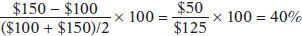
The price elasticity of supply is 50%/40% = 1.25. So supply is elastic.
Question 6.10
True or false? If the demand for milk rose, then, in the long run, milk-drinkers would be better off if supply were elastic rather than inelastic.
True. An increase in demand raises price. If the price elasticity of supply of milk is low, then relatively little additional supply will be forthcoming as the price rises. As a result, the price of milk will rise substantially to satisfy the increased demand for milk. If the price elasticity of supply is high, then a relatively large amount of additional supply will be produced as the price rises. As a result, the price of milk will rise only by a little to satisfy the higher demand for milk.
Question 6.11
True or false? Long-run price elasticities of supply are generally larger than short-run price elasticities of supply. As a result, the short-run supply curves are generally flatter than the long-run supply curves.
False. It is true that long-run price elasticities of supply are generally larger than short-run elasticities of supply. But this means that the short-run supply curves are generally steeper, not flatter, than the long-run supply curves.
Question 6.12
True or false? When supply is perfectly elastic, changes in demand have no effect on price.
True. When supply is perfectly elastic, the supply curve is a horizontal line. So a change in demand has no effect on price; it affects only the quantity bought and sold.