In making any type of decision, it’s critical to define the costs and benefits of that decision accurately. If you don’t know the costs and benefits, it is nearly impossible to make a good decision. So that is where we begin.

An important first step is to recognize the role of opportunity cost, a concept we first encountered in Chapter 1, where we learned that opportunity costs arise because resources are scarce. Because resources are scarce, the true cost of anything is what you must give up to get it—its opportunity cost.

Whether you decide to continue in school for another year or leave to find a job, each choice has costs and benefits. Because your time—a resource—is scarce, you cannot be both a full-time student and a full-time worker. If you choose to be a full-time student, the opportunity cost of that choice is the income you would have earned at a full-time job. And there may be additional opportunity costs, such as the value of the experience you would have gained by working.

When making decisions, it is crucial to think in terms of opportunity cost, because the opportunity cost of an action is often considerably more than the cost of any outlays of money. Economists use the concepts of explicit costs and implicit costs to compare the relationship between opportunity costs and monetary outlays. We’ll discuss these two concepts first. Then we’ll define the concepts of accounting profit and economic profit, which are ways of measuring whether the benefit of an action is greater than the cost. Armed with these concepts for assessing costs and benefits, we will be in a position to consider our first principle of economic decision making: how to make “either–or” decisions.

Suppose that, after graduating from college or university, you have two options: to go to school for an additional year to get an advanced degree or to take a job immediately. You would like to enrol in the extra year in school but are concerned about the cost.

What exactly is the cost of that additional year of school? Here is where it is important to remember the concept of opportunity cost: the cost of the year spent getting an advanced degree includes what you forgo by not taking a job for that year. The opportunity cost of an additional year of school, like any cost, can be broken into two parts: the explicit cost of the year’s schooling and the implicit cost.

An explicit cost is a cost that requires an outlay of money. For example, the explicit cost of the additional year of schooling includes tuition. An implicit cost, though, does not involve an outlay of money; instead, it is measured by the value, in dollar terms, of the benefits that are forgone. For example, the implicit cost of the year spent in school includes the income you would have earned if you had taken a job instead:

A common mistake, both in economic analysis and in life—whether individual or business—is to ignore implicit costs and focus exclusively on explicit costs. But often the implicit cost of an activity is quite substantial—indeed, sometimes it is much larger than the explicit cost.

Table 9-1 gives a breakdown of hypothetical explicit and implicit costs associated with spending an additional year in school instead of taking a job. The explicit cost consists of tuition, books, supplies, and a computer for doing assignments—all of which require you to spend money. The implicit cost is the salary you would have earned if you had taken a job instead. As you can see, the total cost of attending an additional year of schooling is $44 500, the sum of the total implicit cost—$35 000 in forgone salary, and the total explicit cost—$9500 in outlays on tuition, supplies, and computer. Because the implicit cost is more than three times as much as the explicit cost, ignoring the implicit cost would lead to a seriously misguided decision.

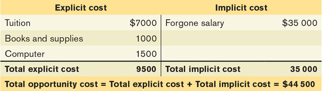
A slightly different way of looking at the implicit cost in this example can deepen our understanding of opportunity cost. The forgone salary is the cost of using your own resources—your time (labour)—in going to school rather than working. The use of your time for more schooling, despite the fact that you don’t have to spend any money on it, is still costly to you. This illustrates an important aspect of opportunity cost: in considering the cost of an activity, you should include the cost of using any of your own resources for that activity. You can calculate the cost of using your own resources by determining what they would have earned in their next best use.

Understanding the role of opportunity costs makes clear the reason for the surge in school applications in 2009 and 2010: a rotten job market. Starting in the fall of 2008, the Canadian job market deteriorated sharply as the economy entered a severe recession. By 2010, the job market was still quite weak; although job openings had begun to reappear, a relatively high proportion of those openings were for jobs with low wages and no benefits. As a result, the opportunity cost of another year of schooling had declined significantly, making spending another year at school a much more attractive choice than when the job market was strong.

Let’s return to Maria from this chapter’s opening story. Assume, hypothetically, that Maria is offered a two-year job in the financial services sector. Also, since she took some university courses in the 1990s, in order to be certified as a social worker, she must complete two years of full-time studies. So she faces the choice of either completing two years of full-time undergraduate studies in social work or spending those two years working in her original field. Which choice should she make?

First, let’s consider what Maria gains by getting the social work degree—what we might call her revenue from the social work degree. Once she has completed her social work degree two years from now, she will receive earnings from her social work degree valued at $600 000 over the rest of her lifetime. In contrast, if she doesn’t get the social work degree and stays in financial services, two years from now her future lifetime earnings will be valued at $500 000. The cost of the tuition for her social work degree program is $40 000, which she pays for with a student loan that costs her $4000 in interest.

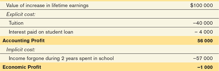
At this point, what she should do might seem obvious: if she chooses the social work degree, she gets a lifetime increase in the value of her earnings of $600 000 − $500 000 = $100 000, and she pays $40 000 in tuition plus $4000 in interest. Doesn’t that mean she makes a profit of $100 000 − $40 000 − $4000 = $56 000 by getting her social work degree? This $56 000 is Maria’s accounting profit from obtaining her social work degree: her revenue minus her explicit cost. In this example her explicit cost of getting the degree is $44 000, the amount of her tuition plus student loan interest:

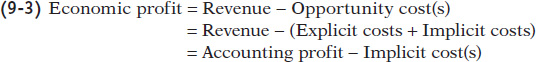
Although accounting profit is a useful measure, it would be misleading for Maria to use it alone in making her decision. To make the right decision, the one that leads to the best possible economic outcome for her, she needs to calculate her economic profit—the revenue she receives from the social work degree minus her opportunity cost of staying in school (which is equal to her explicit cost plus her implicit cost). In general, the economic profit of a given project will be less than the accounting profit because there are almost always implicit costs in addition to explicit costs:

When economists use the term profit, they are referring to economic profit, not accounting profit. This will be our convention in the remainder of the book: when we use the term profit, we mean economic profit.

How does Maria’s economic profit of staying in school differ from her accounting profit? We’ve already encountered one source of the difference: her two years of forgone job earnings. This is an implicit cost of going to school full time for two years. We assume that Maria’s total forgone earnings for the two years is $57 000.

Once we factor in Maria’s implicit costs and calculate her economic profit, we see that she is better off not getting a social work degree. You can see this in Table 9-2: her economic profit from getting the social work degree is −$1000. In other words, she incurs an economic loss of $1000 if she gets the degree. Clearly, she is better off sticking to financial services and going to work now.

To make sure that the concepts of opportunity costs and economic profit are well understood, let’s consider a slightly different scenario. Let’s suppose that Maria does not have to take out $40 000 in student loans to pay her tuition. Instead, she can pay for it with an inheritance from her grandmother. As a result, she doesn’t have to pay $4000 in interest. In this case, her accounting profit is $60 000 rather than $56 000. Would the right decision now be for her to get the social work degree? Wouldn’t the economic profit of the degree now be $60 000 − $57 000 = $3000?

The answer is no, because Maria is using her own capital to finance her education, and the use of that capital has an opportunity cost even when she owns it. Capital is the total value of the assets of an individual or a firm. An individual’s capital usually consists of cash in the bank, stocks, bonds, and the ownership value of real estate such as a house. In the case of a business, capital also includes its equipment, its tools, and its inventory of unsold goods and used parts. (Economists like to distinguish between financial assets, also known as financial capital, such as cash, stocks, and bonds, and physical assets, also known as physical capital, such as buildings, equipment, tools, and inventory.)

The point is that even if Maria owns the $40 000, using it to pay tuition incurs an opportunity cost—what she forgoes in the next best use of that $40 000. If she hadn’t used the money to pay her tuition, her next best use of the money would have been to deposit it in a bank to earn interest. To keep things simple, let’s assume that she earns $4000 on that $40 000 once it is deposited in a bank. Now, rather than pay $4000 in explicit costs in the form of student loan interest, Maria pays $4000 in implicit costs from the forgone interest she could have earned.

This $4000 in forgone interest earnings is what economists call the implicit cost of capital—the income the owner of the capital could have earned if the capital had been employed in its next best alternative use. The net effect is that it makes no difference whether Maria finances her tuition with a student loan or by using her own funds. This comparison reinforces how carefully you must keep track of opportunity costs when making a decision.

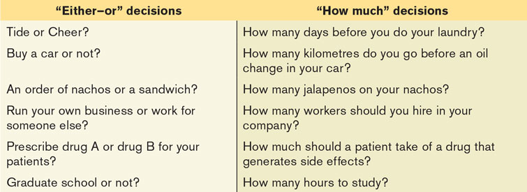
An “either–or” decision is one in which you must choose between two activities. Since doing one precludes you from doing the other, the choice is really between alternative A or alternative B. That’s in contrast to a “how much” decision, which requires you to choose how much of a given activity to undertake. For example, Maria faced an “either–or” decision: to spend two years obtaining a social work degree, or to work. In contrast, a “how much” decision would be deciding how many hours to study or how many hours to work at a job. Table 9-3 contrasts a variety of “either–or” and “how much” decisions.

In making economic decisions, as we have already emphasized, it is vitally important to calculate opportunity costs correctly. The best way to make an “either–or” decision, the method that leads to the best possible economic outcome, is the straightforward principle of “either–or” decision making. According to this principle, when making an “either–or” choice between two activities, choose the one with the positive economic profit. In other words, we should do an activity only if its benefit outweighs its opportunity cost.

Let’s examine Maria’s dilemma from a different angle to understand how this principle works. First, recall Equation 9-3: the economic profit of an alternative is the revenue that choice brings minus the opportunity cost(s) of its alternative (the opportunity costs consist of both explicit and implicit costs). If Maria continues with financial services and goes to work immediately, the total value of her lifetime earnings (her revenue) is $57 000 (her earnings over the next two years) + $500 000 (the value of her lifetime earnings thereafter) = $557 000. Going to work immediately involves no explicit costs, but she does incur implicit costs. Let’s consider those implicit costs.

If she gets her social work degree instead and works in that field, the total value of her lifetime earnings (net of explicit costs) is $600 000 (value of her lifetime earnings after two years in school) − $40 000 (tuition) − $4000 (interest payments) = $556 000. So by going to work immediately, rather than school, her implicit cost is the forgone $556 000. Therefore the economic profit from continuing in financial services versus becoming a social worker is $557 000 − $556 000 = $1000.

So the right choice for Maria is to begin work in financial services immediately, since this gives her an economic profit of $1000, rather than become a social worker, which would give her an economic profit of −$1000.¹ In other words, by becoming a social worker she loses the $1000 economic profit she would have gained by working in financial services immediately.

When choosing between a pair of alternatives, notice that the economic profit of one alternative is always the opposite of the economic profit of the other. This is a general principle, so having calculated the economic profit of one alternative we immediately know the economic profit of the other alternative by using symmetry:

In making “either–or” decisions, mistakes most commonly arise when people or businesses use their own assets in projects rather than rent or borrow assets. That’s because they fail to account for the implicit cost of using self-owned capital. In contrast, when they rent or borrow assets, these rental or borrowing costs show up as explicit costs. If, for example, a restaurant owns its equipment and tools, it would have to compute its implicit cost of capital by calculating how much the equipment could be sold for and how much could be earned by using those funds in the next best alternative project. In addition, businesses run by the owner (an entrepreneur) often fail to calculate the opportunity cost of the owner’s time in running the business. In that way, small businesses often underestimate their opportunity costs and overestimate their economic profit of staying in business.

Are we implying that the hundreds of thousands who have chosen to go back to school rather than find work in recent years are misguided? Not necessarily. As we mentioned before, the poor job market had greatly diminished the opportunity cost of forgone wages for many students, making continuing their education the optimal choice for them.

The following Economics in Action illustrates just how important it is in real life to understand the difference between accounting profit and economic profit.