Section 1 Elasticity of Demand

5.1 The price elasticity of demand measures how sensitive consumers are to changes in price.

What Do the E_d Numbers Mean?

5.2 E_d > 1: Elastic Demand (many substitutes, high-priced goods, longer time horizon, luxury goods)
E_d < 1: Inelastic Demand (few substitutes, low-priced goods, shorter time horizon, necessities)
E_d = 1: Unitary Elastic Demand (a change in price results in an equal percentage change in quantity demanded)

Determinants of Elasticity of Demand

5.3

The formula for price elasticity of demand is

5.4

E_d = % Change in Quantity Demanded/% Change in Price

Since all E_d must be negative according to the law of demand, the convention is to drop the negative sign.

Calculating percentage changes:

Base method: percentage Change in P = Change in P/old P

The base method is simple because it is how one normally calculates percentages in everyday life, such as for store discounts or restaurant tips. For example, adding a 15% tip to a $20 bill is $3, or taking 25% off of a $40 shirt makes the shirt $30.

Midpoint method: % Change in P = Change in P/[(old P + new P)/2]

The midpoint method is slightly more difficult to calculate; however, the advantage is that the percentage change stays the same whether a value increases or decreases. For example, using the midpoint method, going from 10 to 20 or from 20 to 10 is a 66.7% change in either direction.

How Do You Remember Which Diagram Is Elastic?

Think of a pair of shorts: You can easily pull them side-to-side because the waistband is very elastic!

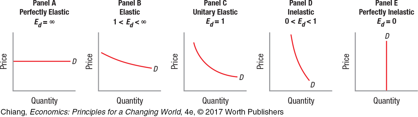
The flatter the demand curve, the more elastic the demand for the good or service; the steeper the demand curve, the more inelastic the demand for the good or service. Because elasticity changes along a linear demand curve, unitary elastic demand has a curved shape.

130

Section 2

Total Revenue and Other
Measures of Elasticity

5.5 Total revenue is calculated as Price × Quantity Demanded.

Total revenue increases when price rises on an inelastic good or is lowered on an elastic good.

Total revenue decreases when price rises on an elastic good or is lowered on an inelastic good.

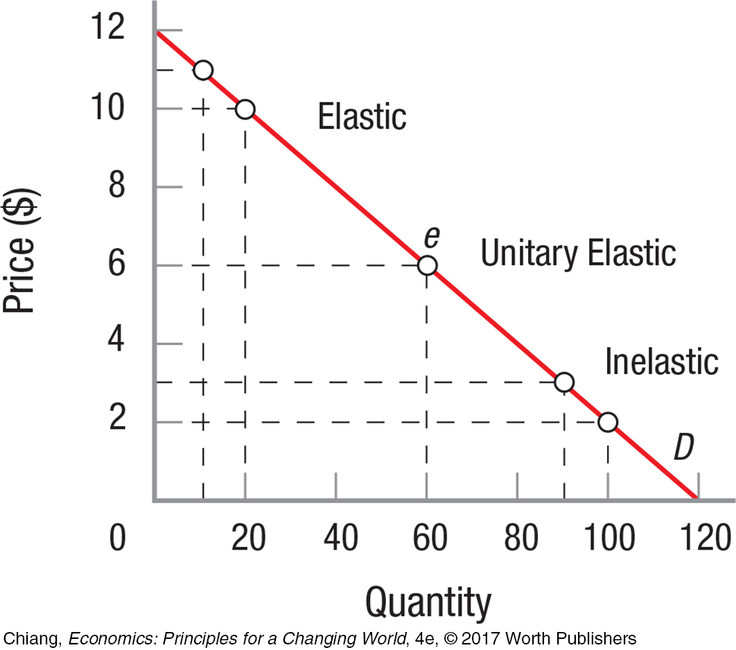
Elasticity and total revenue vary along a straight-line demand curve. Total revenue is maximized at the point where demand is unitary elastic.

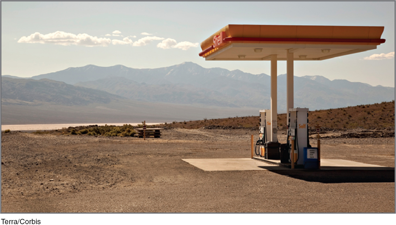
When competition is nearly nonexistent, sellers can raise prices and increase total revenue because the good is inelastic.

5.6 Cross elasticity of demand measures how responsive demand for one good is to a change in the price of another good:

E_ab = % Change in Q_a/% Change in P_b
E_ab > 0: Goods a and b are substitutes.
E_ab < 0: Goods a and b are complements.
E_ab = 0: Goods a and b are unrelated.

5.7 Income elasticity of demand measures how demand demand responds to changes in income: E_Y = % Change in Q/% Change in Income.
0 < E_Y < 1: normal good
E_Y > 1: luxury good
E_Y < 0: inferior good

Section 3 Elasticity of Supply

5.8 The elasticity of supply measures the extent to which businesses react to price changes, and its formula is virtually identical to that of demand:

E_S = % Change in Quantity Supplied / % Change in Price

The base and midpoint methods are both still used to calculate % changes.

5.9 The time horizon affects the elasticity of supply: The longer the period, the more a firm is able to adjust to changing prices, and therefore the more elastic the good.

Short run: a time period in which plant capacity is fixed and the number of firms in an industry does not change.

Long run: a time period long enough for firms to alter their plant capacity or for firms to enter or leave the industry.

Section 4 Taxes and Elasticity

5.10 The incidence of taxation refers to who bears the economic burden of a tax.

The more elastic the demand or inelastic the supply, the greater the incidence of a tax on sellers. The more inelastic the demand or elastic the supply, the greater the incidence of a tax on consumers.

A new tax collected on sellers shifts the supply curve to the left. The intersection of S_{0 + tax} and D₀ determines the price consumers pay, P_C. P_S is the price sellers receive. The difference between P_C and P_S is the tax per unit.

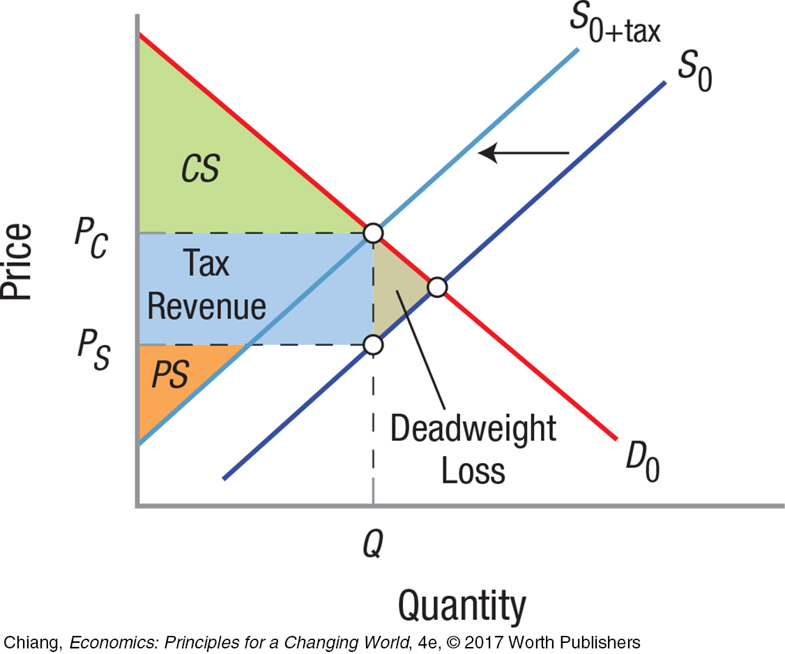
The tax created a deadweight loss shown in gray, along with a reduction in consumer surplus (CS) and producer surplus (PS). The government collects tax revenue shown as the area in blue.