DEMAND
Whenever you purchase a product, you are voting with your money. You are selecting one product out of many and supporting one firm out of many, both of which signal to the business community what sorts of products satisfy your wants as a consumer.
Economists typically focus on wants rather than needs because it is so difficult to determine what we truly need. Theoretically, you could survive on tofu and vitamin pills, living in a lean-
Willingness-
willingness-
Imagine sitting in your economics class around mealtime. In your rush to class, you did not have a chance to make a sandwich at home or to stop at the cafeteria on your way to class. You think about foods that sound appealing to you (just about anything at this point), and plan to go to the cafeteria immediately after class and buy a sandwich. Given your growling stomach, you think more about what you want on your sandwich and less about how much the sandwich will cost. In your mind, your willingness-
58
Economists refer to WTP as the maximum amount one would be willing to pay for a good or service, which represents the highest value that a consumer believes the good or service is worth. Of course, one always hopes that the actual price would be much lower. In your case, WTP is the cutoff between buying a sandwich and not buying a sandwich.
WTP varies from person to person, from the circumstances each person is in to the number of sandwiches one chooses to buy. Suppose your classmate ate a full meal before she came to class. Her WTP for a sandwich would be much lower than yours because she isn’t hungry at that moment. Similarly, after you buy and consume your first sandwich, your WTP for a second sandwich would decrease because you would be less hungry. The desires consumers have for goods and services are expressed through their purchases in the market.
Figure 1 illustrates how individuals’ WTP is used to derive market demand curves. Suppose you are willing to pay up to $10 for the first sandwich and $4 for the second sandwich (shown in panel A), while Jane, your less-
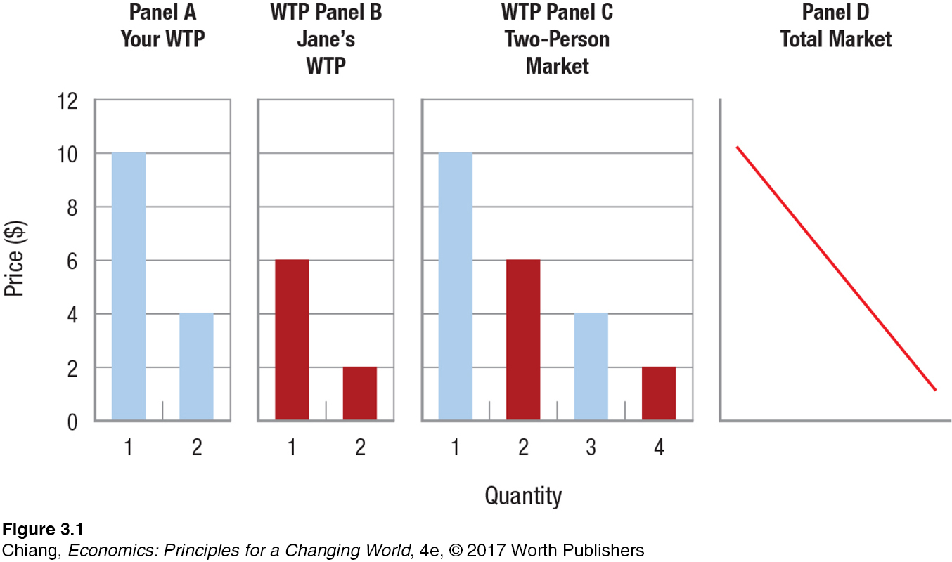
These illustrations show how ordinary demand curves, which we will discuss in detail in the remainder of this section, are developed from the perceptions of what individual consumers believe a good or service is worth to them (their WTP). Let’s now discuss an important characteristic of market demand.
The Law of Demand: The Relationship Between Quantity Demanded and Price
demand The maximum amount of a product that buyers are willing and able to purchase over some time period at various prices, holding all other relevant factors constant (the ceteris paribus condition).
Demand refers to the goods and services people are willing and able to buy during a certain period of time at various prices, holding all other relevant factors constant (the ceteris paribus condition). Typically, when the price of a good or service increases (say your favorite café raises its prices), the quantity demanded will decrease because fewer and fewer people will be willing and able to spend their money on such things. However, when prices of goods or services decrease (think of sales offered the day after Thanksgiving), the quantity demanded increases.
59
In a market economy, there is a negative relationship between price and quantity demanded. This relationship, in its most basic form, states that as price increases, the quantity demanded falls, and conversely, as price falls, the quantity demanded increases.
law of demand Holding all other relevant factors constant, as price increases, quantity demanded falls, and as price decreases, quantity demanded rises.
This principle, when all other factors are held constant, is known as the law of demand. The law of demand states that the lower a product’s price, the more of that product consumers will purchase during a given time period. This straightforward, commonsense notion happens because, as a product’s price drops, consumers will substitute the now cheaper product for other, more expensive products. Conversely, if the product’s price rises, consumers will find other, less expensive products to substitute for it.
To illustrate, when videocassette recorders first came on the market 35 years ago, they cost $3,000, and few homes had one. As VCRs became less and less expensive, however, more people bought them, and others found more uses for them. Two decades later, VCRs became obsolete as DVD players became the standard means of watching movies at home. Today, DVD players are becoming obsolete as digital movie streaming surpassed DVD sales. Similarly, digital music players have altered the structure of the music business, and digital cameras have essentially replaced cameras that use film.
Time is an important component in the demand for many products. Consuming many products—
The Demand Curve
demand curve A graphical illustration of the law of demand, which shows the relationship between the price of a good and the quantity demanded.
The law of demand states that as price decreases, quantity demanded increases. When we translate demand information into a graph, we create a demand curve. This demand curve, which slopes down and to the right, graphically illustrates the law of demand. A demand curve shows both the willingness-
Consider the market for gaming apps, games that can be downloaded onto one’s smartphone or tablet. The mobile gaming industry is a $25 billion industry. Although each gaming app costs no more than a few dollars to download, sales of gaming apps have surpassed sales of PC and console games. Gaming apps such as Candy Crush Saga, Angry Birds, and Words with Friends have each been downloaded hundreds of millions of times. Let’s examine the relationship between the price of gaming apps and the quantity demanded by individual consumers and the market. For simplicity, assume that all gaming apps are the same price.
demand schedule A table that shows the quantity of a good a consumer purchases at each price.
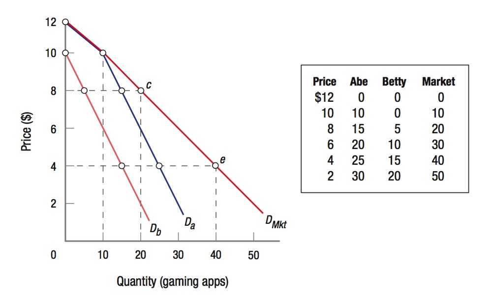
Suppose Abe and Betty are the only two consumers in the market for gaming apps. Figure 2 shows each of their annual demands using a demand schedule and a demand curve. A demand schedule is a table indicating the quantities consumers are willing to purchase at each price. Looking at the demand schedule, we can see that both Abe and Betty are willing to buy more gaming apps as the price decreases. When the price is $10, Abe is willing to buy 10 games, while Betty buys none. When the price falls to $8, Abe is willing to buy 15 games and Betty would buy 5.
We can take the values from the demand schedule in the table and graph them in a figure, with price shown on the vertical axis and quantity of gaming apps on the horizontal axis, following the convention in economics of always placing price on the vertical axis and quantity on the horizontal axis. By doing so, we can create a demand curve for both Abe and Betty. Both the table and the graph convey the same information. They also both portray the law of demand. As the price decreases, Abe and Betty demand more gaming apps.
horizontal summation The process of adding the number of units of the product purchased or supplied at each price to determine market demand or supply.
60
Although individual demand curves are interesting, market demand curves are far more important to economists, as they can be used to predict changes in product price and quantity. Further, one can observe what happens to a product’s price and quantity and infer what changes have occurred in the market. Market demand is the sum of individual demands. To calculate market demand, economists simply add the number of units of a product all consumers will purchase at each price. This process is known as horizontal summation.
Turning to the demand curves in Figure 2, the individual demand curves for Abe and Betty, Da and Db, are shown. For simplicity, let’s assume they represent the entire market, but recognize that this process would work for any larger number of people. Note that at a price of $10 a game, Betty will not buy any, although Abe is willing to buy 10 apps at $10 each. Above $10, therefore, the market demand is equal to Abe’s demand. At $10 and below, however, we add both Abe’s and Betty’s demands at each price to obtain market demand. Thus, at $8, individual demand is 15 for Abe and 5 for Betty; therefore, the market demand is equal to 20 (point c). When the price is $4 an app, Abe buys 25 and Betty buys 15, for a total of 40 apps (point e). The heavier curve, labeled DMkt, represents this market demand; it is a horizontal summation of the two individual demand curves.
This all sounds simple in theory, but in the real world estimating market demand curves is tricky, given that many markets contain millions of consumers. Economic analysts and marketing professionals use sophisticated statistical techniques to estimate the market demand for particular goods and services in the industries they represent.
The market demand curve shows the maximum amount of a product consumers are willing and able to purchase during a given time period at various prices, all other relevant factors being held constant. Economists use the term determinants of demand to refer to these other, nonprice factors that are held constant. This is another example of the use of ceteris paribus: holding all other relevant factors constant.
Determinants of Demand
determinants of demand Nonprice factors that affect demand, including tastes and preferences, income, prices of related goods, number of buyers, and expectations.
Up to this point, we have discussed only how price affects the quantity demanded. When prices fall, consumers purchase more of a product; thus quantity demanded rises. When prices rise, consumers purchase less of a product; thus, quantity demanded falls. But several other factors besides price also affect demand, including what people like, what their income is, and how much related products cost. More specifically, there are five key determinants of demand: (1) tastes and preferences; (2) income; (3) prices of related goods; (4) the number of buyers; and (5) expectations regarding future prices, income, and product availability. When one of these determinants changes, the entire demand curve changes. Let’s see why.
61
Tastes and Preferences We all have preferences for certain products over others, easily perceiving subtle differences in styling and quality. Automobiles, fashions, phones, and music are just a few of the products that are subject to the whims of the consumer.
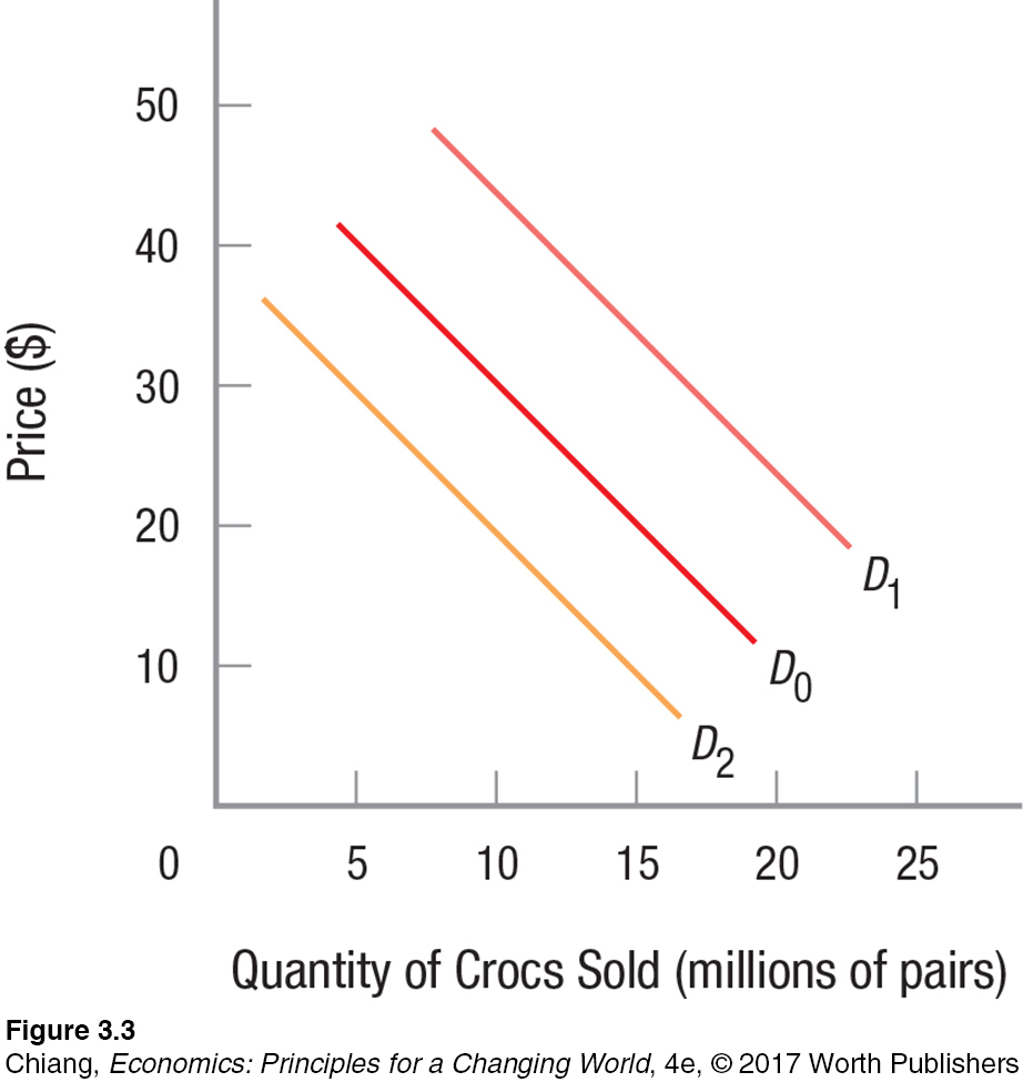
Remember Crocs, those brightly colored rubber sandals with the little air holes that moms, kids, waitresses, and many others favored? They were an instant hit. Initially, demand was D0 in Figure 3. They then became such a fad that demand jumped to D1 and for a short while Crocs were hard to find. Eventually, Crocs were everywhere. Fads come and go, and now the demand for them settled back to something like D2, less than the original level. Notice an important distinction here: More Crocs weren’t sold because the price was lowered; the entire demand curve shifted rightward when they were hot and more Crocs could be sold at all prices. Now that the fad has subsided, fewer will be sold at all prices. It is important to keep in mind that when one of the determinants changes, such as tastes and preferences, the entire demand curve shifts.
normal good A good for which an increase in income results in rising demand.
Income Income is another important factor influencing consumer demand. Generally speaking, as income rises, demand for most goods will likewise increase. Get a raise, and you are more likely to buy more clothes and acquire the latest technology gadgets. Your demand curve for these goods will shift to the right (such as from D0 to D1 in Figure 3). Products for which demand is positively linked to income—
inferior good A good for which an increase in income results in declining demand.
There are also some products for which demand declines as income rises, and the demand curve shifts to the left. Economists call these products inferior goods. As income grows, for instance, the consumption of discount clothing and cheap motel stays will likely fall as individuals upgrade their wardrobes and stay in more comfortable hotels when traveling. Similarly, when you graduate from college and your income rises, your consumption of ramen noodles will fall as you begin to cook tastier dinners and eat out more frequently.
substitute goods Goods consumers will substitute for one another. When the price of one good rises, the demand for the other good increases, and vice versa.
Prices of Related Goods The prices of related commodities also affect consumer decisions. You may be an avid concertgoer, but with concert ticket prices often topping $100, further rises in the price of concert tickets may entice you to see more movies and fewer concerts. Movies, concerts, plays, and sporting events are good examples of substitute goods, because consumers can substitute one for another depending on their respective prices. When the price of concerts rises, your demand for movies increases, and vice versa. These are substitute goods.
complementary goods Goods that are typically consumed together. When the price of a complementary good rises, the demand for the other good declines, and vice versa.
62
Movies and popcorn, on the other hand, are examples of complementary goods. These are goods that are generally consumed together, such that an increase or decrease in the consumption of one will similarly result in an increase or decrease in the consumption of the other—
The Number of Buyers Another factor influencing market demand for a product is the number of potential buyers in the market. Clearly, the more consumers there are who would be likely to buy a particular product, the higher its market demand will be (the demand curve will shift rightward). As our average life span steadily rises, the demands for medical services and retirement communities likewise increases. As more people than ever enter universities and graduate schools, demand for textbooks and backpacks increases.
Expectations About Future Prices, Incomes, and Product Availability The final factor influencing demand involves consumer expectations. If consumers expect shortages of certain products or increases in their prices in the near future, they tend to rush out and buy these products immediately, thereby increasing the present demand for the products. The demand curve shifts to the right. During the Florida hurricane season, when a large storm forms and begins moving toward the coast, the demand for plywood, nails, bottled water, and batteries quickly rises.
The expectation of a rise in income, meanwhile, can lead consumers to take advantage of credit in order to increase their present consumption. Department stores and furniture stores, for example, often run “no payments until next year” sales designed to attract consumers who want to “buy now, pay later.” These consumers expect to have more money later, when they can pay, so they go ahead and buy what they want now, thereby increasing the present demand for the promoted items. Again, the demand curve shifts to the right.
The key point to remember from this section is that when one of the determinants of demand changes, the entire demand curve shifts rightward (an increase in demand) or leftward (a decline in demand). A quick look back at Figure 3 shows that when demand increases, consumers are willing to buy more at all prices, and when demand decreases, they will buy less at each and every price.
Changes in Demand Versus Changes in Quantity Demanded
When the price of a product rises, consumers buy fewer units of that product. This is a movement along an existing demand curve. However, when one or more of the determinants changes, the entire demand curve is altered. Now at any given price, consumers are willing to purchase more or less depending on the nature of the change. This section focuses on this important distinction between changes in demand versus changes in quantity demanded.
change in demand Occurs when one or more of the determinants of demand changes, shown as a shift in the entire demand curve.
A change in demand occur whenever one or more of the determinants of demand change and demand curves shift. When demand changes, the demand curve shifts either to the right or to the left. Let’s look at each shift in turn.
Demand increases when the entire demand curve shifts to the right. At all prices, consumers are willing to purchase more of the product in question. Figure 4 shows an increase in demand for gaming apps; the demand curve shifts from D0 to D1. Notice that more gaming apps are purchased at all prices along D1 as compared to D0.
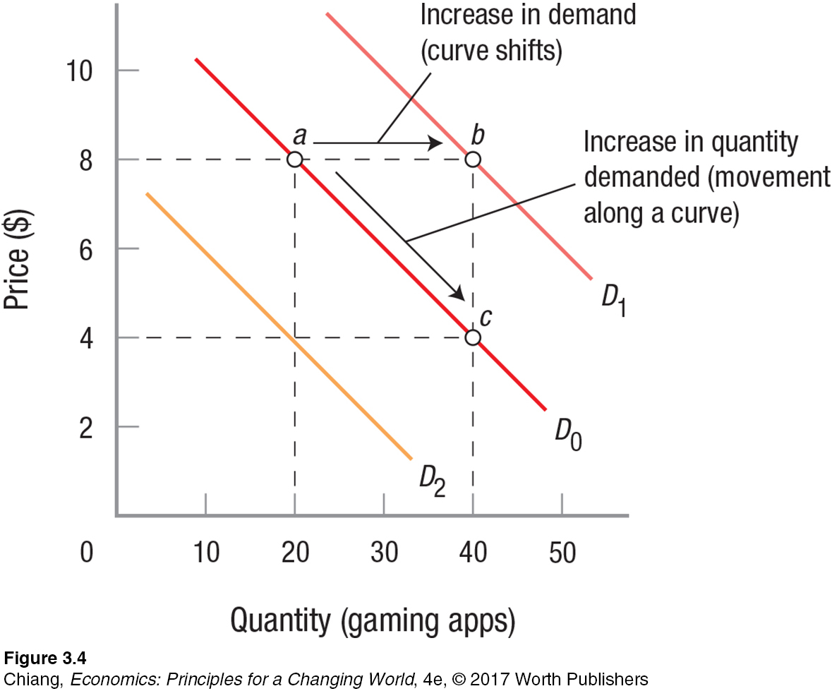
Now look at a decrease in demand, when the entire demand curve shifts to the left. At all prices, consumers are willing to purchase less of the product in question. A drop in consumer income is normally associated with a decrease in demand (the demand curve shifts to the left, as from D0 to D2 in Figure 4).
change in quantity demanded Occurs when the price of the product changes, shown as a movement along an existing demand curve.
63
Whereas a change in demand can be brought about by many different factors, a change in quantity demanded can be caused by only one thing: a change in product price. This is shown in Figure 4 as a reduction in price from $8 to $4, resulting in sales (quantity demanded) increasing from 20 (point a) to 40 (point c) apps. This distinction between a change in demand and a change in quantity demanded is important. Reducing price to increase sales is different from spending a few million dollars on Super Bowl advertising to increase sales at all prices.
These concepts are so important that a quick summary is in order. As Figure 4 illustrates, given the initial demand D0, increasing sales from 20 to 40 apps can occur in either of two ways. First, changing a determinant (say, increasing advertising) could shift the demand curve to D1 so that 40 apps would be sold at $8 (point b). Alternatively, 40 apps could be sold by reducing the price to $4 (point c). Selling more by increasing advertising causes an increase in demand, or a shift in the entire demand curve. Simply reducing the price, on the other hand, causes an increase in quantity demanded, or a movement along the existing demand curve, D0, from point a to point c.
CHECKPOINT
DEMAND
A person’s willingness-
to- pay is the maximum amount she or he values a good to be worth at a particular moment in time and is the building block for demand. Demand refers to the quantity of products people are willing and able to purchase at various prices during some specific time period, all other relevant factors being held constant.
The law of demand states that price and quantity demanded have an inverse (negative) relation. As price rises, consumers buy fewer units; as price falls, consumers buy more units. It is depicted as a downward-
sloping demand curve. Demand curves shift when one or more of the determinants of demand change.
The determinants of demand are consumer tastes and preferences, income, prices of substitutes and complements, the number of buyers in a market, and expectations about future prices, incomes, and product availability.
A shift of a demand curve is a change in demand, and occurs when a determinant of demand changes.
A change in quantity demanded occurs only when the price of a product changes, leading consumers to adjust their purchases along the existing demand curve.
64
QUESTIONS: Sales of electric plug-
Answers to the Checkpoint questions can be found at the end of this chapter.
The ability to avoid high gasoline prices, a general rise in environmental consciousness, incentives such as preferred parking and reduced tolls offered by some states, an increase in the availability of charging stations (reducing opportunity cost), and improvements in quality have all led to an increase in demand for plug-