MARKET EQUILIBRIUM
equilibrium Market forces are in balance when the quantities demanded by consumers just equal the quantities supplied by producers.
equilibrium price The price at which the quantity demanded is just equal to quantity supplied.
equilibrium quantity The output that results when quantity demanded is just equal to quantity supplied.
Supply and demand together determine the prices and quantities of goods bought and sold. Neither factor alone is sufficient to determine price and quantity. It is through their interaction that supply and demand do their work, just as two blades of a scissors are required to cut paper.
A market will determine the price at which the quantity of a product demanded is equal to the quantity supplied. At this price, the market is said to be cleared or to be in equilibrium, meaning that the amount of the product that consumers are willing and able to purchase is matched exactly by the amount that producers are willing and able to sell. This is the equilibrium price and the equilibrium quantity. The equilibrium price is also called the market-
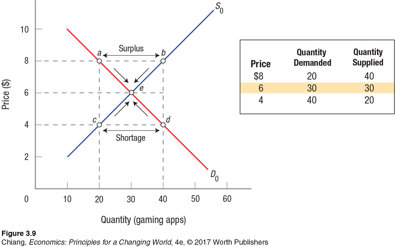
Figure 9 puts together Figures 2 and 5, showing the market supply and demand for gaming apps. It illustrates how supply and demand interact to determine equilibrium price and quantity. Clearly, the quantities demanded and supplied equal one another only where the supply and demand curves cross, at point e. From the table in Figure 9, you can see that quantity demanded and quantity supplied are the same at only one price. At $6 per app, sellers are willing to provide exactly the same quantity as consumers would like to purchase. Hence, at this price, the market clears, since buyers and sellers both want to transact the same number of units.
surplus Occurs when the price is above market equilibrium, and quantity supplied exceeds quantity demanded.
The beauty of a market is that it automatically works to establish the equilibrium price and quantity, without any guidance from anyone. To see how this happens, let us assume that gaming apps are initially priced at $8, a price above their equilibrium price. As we can see by comparing points a and b, sellers are willing to supply more apps at this price than consumers are willing to buy. Economists characterize such a situation as one of excess supply, or surplus. In this case, at $8, sellers supply 40 apps to the market (point b), yet buyers want to purchase only 20 (point a). This leaves an excess of 20 apps overhanging the market; these unsold apps ultimately become surplus inventories.
70
Here is where the market kicks in to restore equilibrium. As inventories rise, most firms cut production. Some firms, moreover, start reducing their prices to increase sales. Other firms must then cut their own prices to remain competitive. This process continues, with firms cutting their prices and production, until most firms have managed to exhaust their surplus inventories. This happens when prices reach $6 and quantity supplied equals 30, because consumers are once again willing to buy up the entire quantity supplied at this price, and the market is restored to equilibrium.
shortage Occurs when the price is below market equilibrium, and quantity demanded exceeds quantity supplied.
In general, therefore, when prices are set too high, surpluses result, which drive prices back down to their equilibrium levels. If, conversely, a price is initially set too low, say, at $4, a shortage results. In this case, buyers want to purchase 40 apps (point d), but sellers are only providing 20 (point c), creating a shortage of 20 apps. Because consumers are willing to pay more than $4 to obtain the few apps available on the market, they will start bidding up the price of gaming apps. Sensing an opportunity to make some money, firms will start raising their prices and increasing production once again until equilibrium is restored. Hence, in general, excess demand causes firms to raise prices and increase production.
When there is a shortage in a market, economists speak of a tight market or a seller’s market. Under these conditions, producers have no difficulty selling off all their output. On the other hand, when a surplus of goods floods the market, this gives rise to a buyer’s market, because buyers can buy all the goods they want at attractive prices.
We have now seen how changing prices naturally works to clear up shortages and surpluses, thereby returning markets to equilibrium. Some markets, once disturbed, will return to equilibrium quickly. Examples include the stock, bond, and money markets, where trading is nearly instantaneous and extensive information abounds. Other markets react very slowly. Consider the labor market, for instance. When workers lose their jobs due to a plant closing, most will search for new jobs that pay at least as much as the salary at their previous jobs. Some will be successful, while others might struggle, having to settle for a lower-
These automatic market adjustments can make some buyers and sellers feel uncomfortable: It seems as if prices and quantities are being set by forces beyond anyone’s control. In fact, this phenomenon is precisely what makes market economies function so efficiently. Without anyone needing to be in control, prices and quantities naturally gravitate toward equilibrium levels. Adam Smith was so impressed by the workings of the market that he suggested that it is almost as if an “invisible hand” guides the market to equilibrium.
71
Given the self-
ALFRED MARSHALL (1842–1924)
British economist Alfred Marshall is considered the father of the modern theory of supply and demand—
With financial help from his uncle, Marshall attended St. John’s College, Cambridge, to study mathematics and physics. However after long walks through the poorest sections of several European cities and seeing their horrible conditions, he decided to focus his attention on political economy.
In 1890 he published Principles of Economics. In it he introduced many new ideas, though he would never boast about them as being novel. In hopes of appealing to the general public, Marshall buried his diagrams in footnotes. And, although he is credited with many economic theories, he would always clarify them with various exceptions and qualifications. He expected future economists to flesh out his ideas.
Above all, Marshall loved teaching and his students. His lectures were known to never be orderly or systematic because he tried to get students to think with him and ultimately think for themselves. At one point near the turn of the 20th century, essentially all of the leading economists in England had been his students. More than anyone else, Marshall is given credit for establishing economics as a discipline of study. He died in 1924.
Sources: E. Ray Canterbery, A Brief History of Economics: Artful Approaches to the Dismal Science (Hackensack, NJ: World Scientific), 2001; Robert Skidelsky, John Maynard Keynes: Volume 2, The Economist as Saviour 1920–
Moving to a New Equilibrium: Changes in Supply and Demand
Once a market is in equilibrium and the forces of supply and demand balance one another out, the market will remain there unless an external factor changes. But when the supply curve or demand curve shifts (some determinant changes), equilibrium also shifts, resulting in a new equilibrium price and/or output. The ability to predict new equilibrium points is one of the most useful aspects of supply and demand analysis.
Predicting the New Equilibrium When One Curve Shifts When only supply or only demand changes, the change in equilibrium price and equilibrium output can be predicted. We begin with changes in supply.
Changes in Supply Figure 10 shows what happens when supply changes. Equilibrium initially is at point e, with equilibrium price and quantity at $9 and 30, respectively. But let us assume that a rise in wages or the bankruptcy of a key business in the market (the number of sellers falls) causes a decrease in supply. When supply declines (the supply curve shifts from S0 to S2), equilibrium price rises to $12, while equilibrium output falls to 20 (point a).
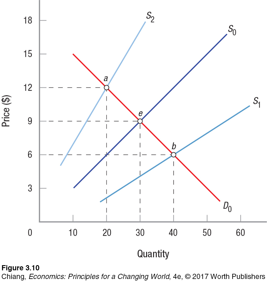
If, on the other hand, supply increases (the supply curve shifts from S0 to S1), equilibrium price falls to $6, while equilibrium output rises to 40 (point b). This is what has happened in the electronics industry: Falling production costs have resulted in more electronic products being sold at lower prices.
72
We have seen how equilibrium price and quantity will change when supply changes. When supply increases, equilibrium price will fall and output will rise; when supply decreases, equilibrium price will rise and output will fall.
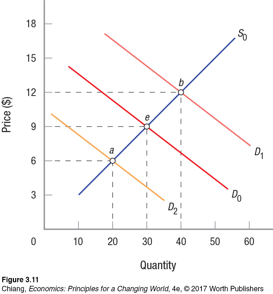
Changes in Demand The effects of demand changes are shown in Figure 11. Again, equilibrium is initially at point e, with equilibrium price and quantity at $9 and 30, respectively. But let us assume that the economy then enters a recession and incomes sink, or perhaps the price of some complementary good soars; in either case, demand falls. As demand decreases (the demand curve shifts from D0 to D2), equilibrium price falls to $6, while equilibrium output falls to 20 (point a).
73
ISSUE
Two-
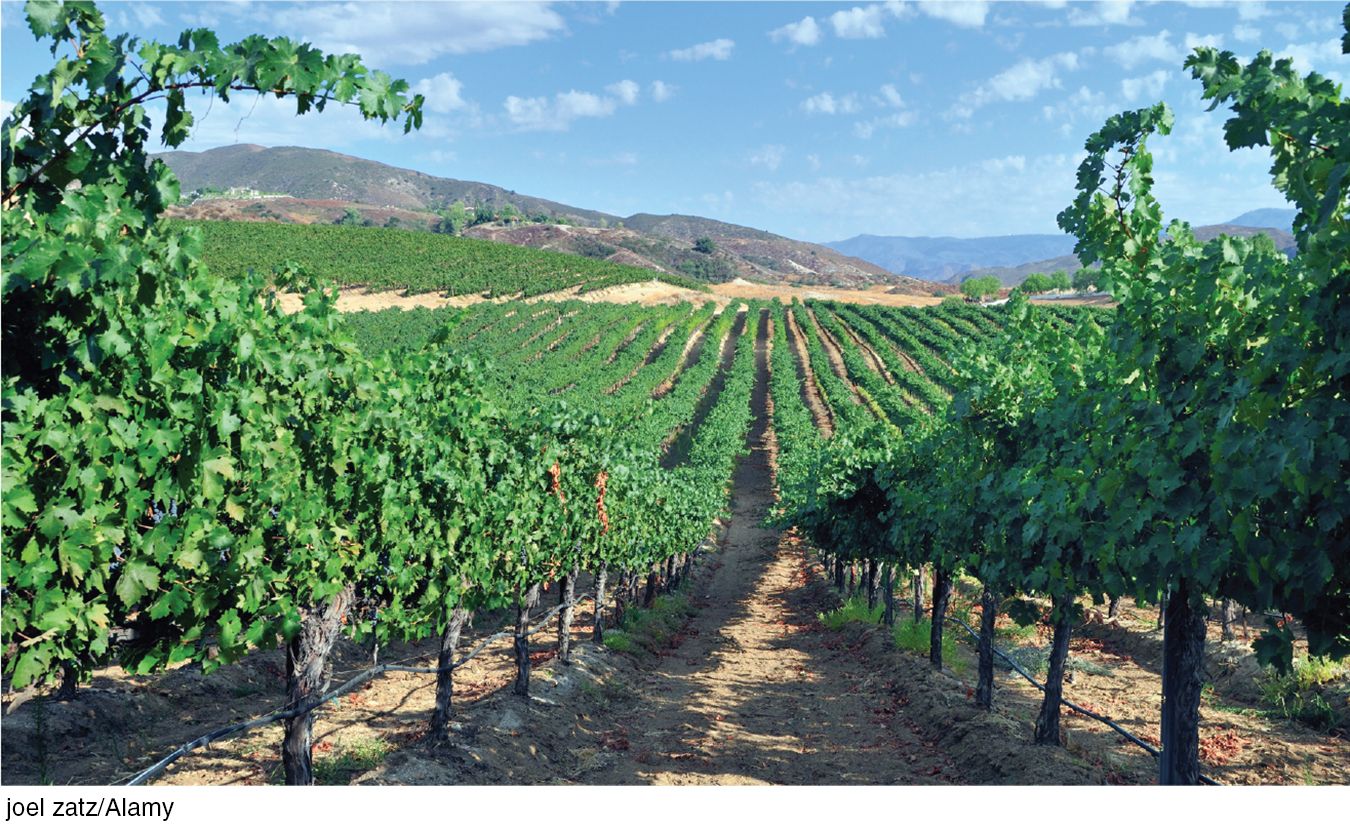
The great California wines of the 1990s put California vineyards on the map. Demand, prices, and exports grew rapidly. Overplanting of new grapevines was a result. When driving along Interstate 5 or Highway 101 north of Los Angeles, one can see vineyards extending for miles, and most were planted in the mid-
Bronco Wine Company president Fred Franzia made an exclusive deal with Trader Joe’s, an unusual supermarket that features innovative food and wine products. He bought the excess grapes at distressed prices, and in his company’s modern plant produced inexpensive wines—
Two-
During the same recession just described, the demand for inferior goods (beans and bologna) will rise, as falling incomes force people to switch to less expensive substitutes. For these products, as demand increases (shifting the demand curve from D0 to D1), equilibrium price rises to $12, and equilibrium output grows to 40 (point b).
Like changes in supply, we can predict how equilibrium price and quantity will change when demand changes. When demand increases, both equilibrium price and output will rise; when demand decreases, both equilibrium price and output will fall.
Predicting the New Equilibrium When Both Curves Shift When both supply and demand change, things get tricky. We can predict what will happen with price in some cases and output in other cases, but not what will happen with both.
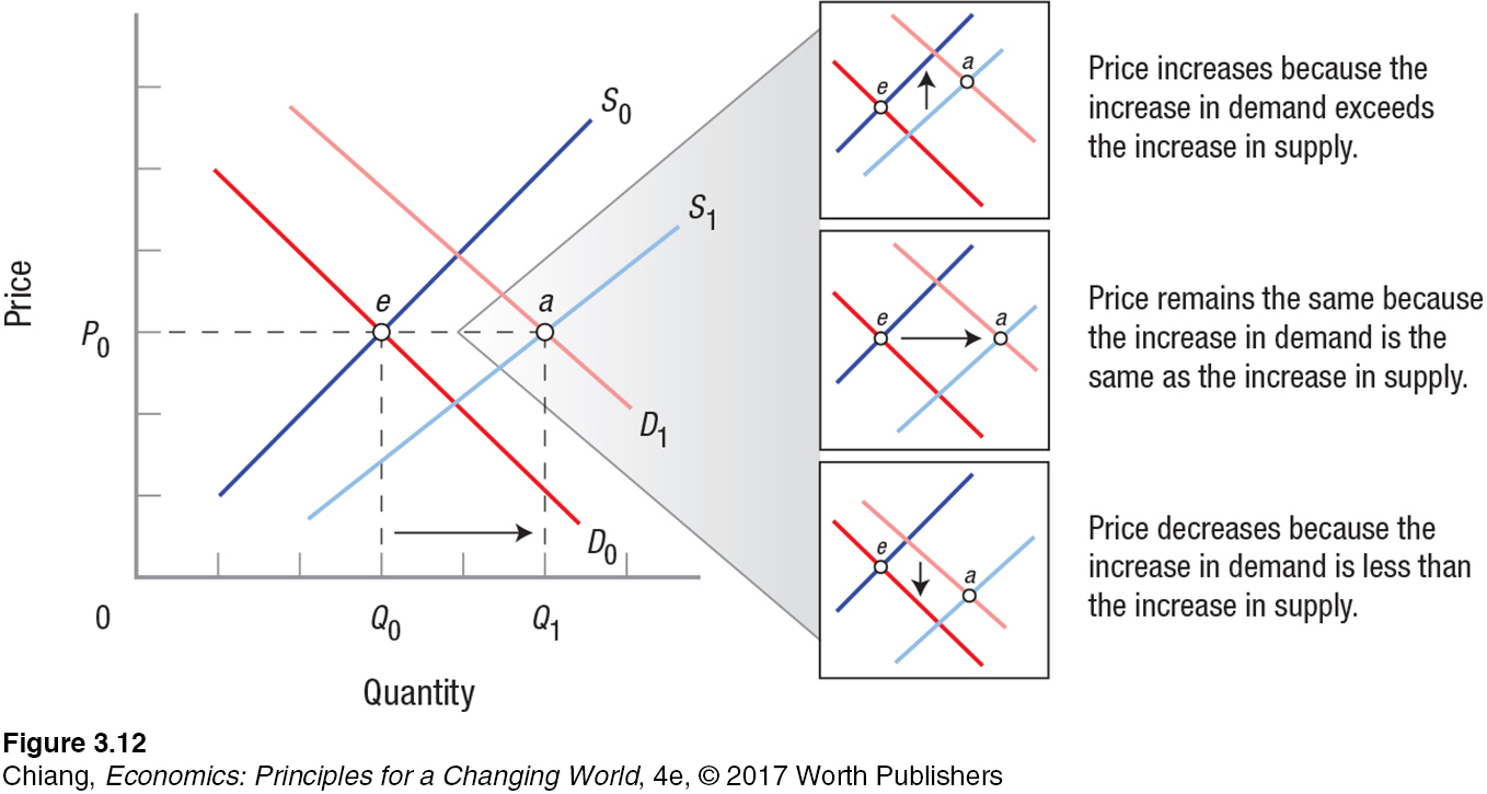
Figure 12 portrays an increase in both demand and supply. Consider the market for corn. Suppose that an increase in corn-
74
But what happens to the price of corn is not so clear. If demand and supply grow the same, output increases, but price remains at P0 (also captured in the middle panel to the right). If demand grows relatively more than supply, the new equilibrium price will be higher (top panel on the right). Conversely, if demand grows relatively less than supply, the new equilibrium price will be lower (bottom panel on the right). Figure 12 is just one of the four possibilities when both supply and demand change. The other three possibilities are shown in Table 1 along with the four possibilities when just one curve shifts. When only one curve shifts, the direction of change in equilibrium price and quantity is certain. But when both curves shift, the direction of change in either the equilibrium price or quantity will be indeterminate.
| TABLE 1 | THE EFFECT OF CHANGES IN DEMAND OR SUPPLY ON EQUILIBRIUM PRICES AND QUANTITIES | |||
| Change in Demand | Change in Supply | Change in Equilibrium Price | Change in Equilibrium Quantity | |
| One Curve Shifting | No change | Increase | Decrease | Increase |
| No change | Decrease | Increase | Decrease | |
| Increase | No change | Increase | Increase | |
| Decrease | No change | Decrease | Decrease | |
| Both Curves Shifting | Increase | Increase | Indeterminate | Increase |
| Decrease | Decrease | Indeterminate | Decrease | |
| Increase | Decrease | Increase | Indeterminate | |
| Decrease | Increase | Decrease | Indeterminate | |
75
Tokyo Disneyland: Is THAT the Line for Space Mountain?!
What are some factors that cause Tokyo Disneyland to be so crowded even during the middle of winter?
How long are you willing to wait to experience your favorite ride at a theme park? 20 minutes? 60 minutes? How about 3 hours? On an ordinary day at Tokyo Disneyland, one of the most popular theme parks in the world, the line for its famous attractions such as Space Mountain, Splash Mountain, and Tower of Terror can reach 200 minutes…. That’s over a 3-
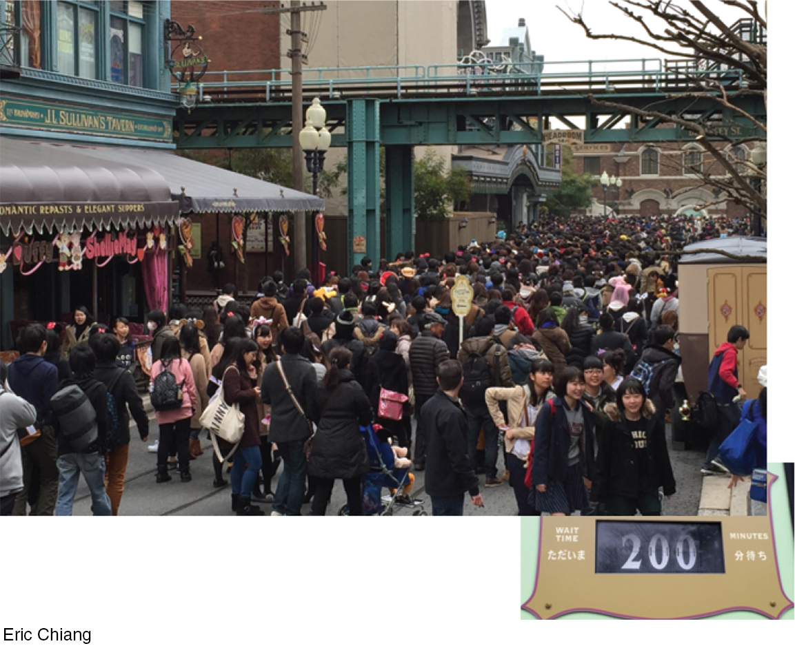
Theme park rides have lines because the quantity of rides demanded exceeds the quantity supplied. Why is that? Because most theme parks charge a fixed admission fee for unlimited rides, visitors typically demand more rides than the theme park is able to supply, even if a ride is operating at full capacity. The extent of the shortage, and consequently the length of wait time, are influenced largely by market factors.
First, consider the role of preferences. Disneyland has a worldwide following, and for those living in Japan, visiting Tokyo Disneyland is certainly easier than visiting Disney parks in California or Florida. Second, consider the number of potential buyers. Tokyo Disneyland is located in a metropolitan area with over 30 million people. The sheer number of potential visitors will lead to higher demand. And third, consider the role of pricing. Given its popularity, Tokyo Disneyland could charge higher prices to reduce the quantity demanded. Yet, in 2016 a one-
The combination of preferences, proximity to potential buyers, and relatively low prices cause demand for Tokyo Disneyland rides to far exceed the park’s reasonable capacity (at least by U.S. standards), creating massive lines. Yet for enthusiastic Disney fans, smiling faces abound. Despite the crowds, it’s still the “Happiest Place on Earth!”
GO TO  TO PRACTICE THE ECONOMIC CONCEPTS IN THIS STORY
CHECKPOINT
MARKET EQUILIBRIUM
Together, supply and demand determine market equilibrium, which occurs when the quantity supplied exactly equals quantity demanded.
The equilibrium price is also called the market-
clearing price. When quantity demanded exceeds quantity supplied, a shortage occurs and prices are bid up toward equilibrium. When quantity supplied exceeds quantity demanded, a surplus occurs and prices are pushed down toward equilibrium.
When supply and demand change, equilibrium price and output change.
When only one curve shifts, the resulting changes in equilibrium price and quantity can be predicted.
When both curves shift, we can predict the change in equilibrium price in some cases or the change in equilibrium quantity in others, but never both. We have to determine the relative magnitudes of the shifts before we can predict both equilibrium price and quantity.
QUESTIONS: In China, where lines are a routine part of everyday life, a growing industry of professional line waiters has developed. Exactly as it sounds, these people are paid an average of $3 an hour to wait in line for others, a wage that is higher than what a typical factory worker in China earns. Today, the professional line waiter has popped up in cities around the world, including New York, though at significantly higher prices than in China. Given that one can pay someone to wait, what might happen in the market for goods and services most prone to long waiting lines, such as prime concert tickets or the latest technology gadget?
Answers to the Checkpoint questions can be found at the end of this chapter.
Waiting in line for a new product or a good deal adds to the cost of acquiring a good. For those with higher opportunity costs of time, hiring a professional line waiter reduces this cost, making the product more affordable. Therefore, professional line waiters would cause an increase in demand for goods and services more prone to lines, causing even greater lines and shortages if prices do not adjust upward.