So far, we have looked at the consumer when we studied the elasticity of demand. Now let us turn our attention to the producer, and analyze elasticity of supply.

Price elasticity of supply (E_s) measures the responsiveness of quantity supplied to changes in the price of the product. Price elasticity of supply is defined as

Note that because the slope of the supply curve is positive, the price elasticity of supply will always be a positive number. Economists classify price elasticity of supply in the same way that they classify price elasticity of demand. Classification is based on whether the percentage change in quantity supplied is greater than, less than, or equal to the percentage change in price. When price rises just a little and quantity increases by much more, supply is elastic, and vice versa. The output of many commodities such as gold and seasonal vegetables cannot be quickly increased if their price increases, so they are inelastic. In summary,

elastic supply: E_s > 1

Inelastic supply: E_s < 1

Unitary elastic supply: E_s = 1

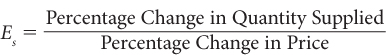
Looking at the three supply curves in Figure 5, we can easily determine which curve is inelastic, which is elastic, and which is unitary elastic. First, note that all three curves go through point a. As we increase the price from P₀ to P₁, we see that the response in quantity supplied is different for all three curves. Consider supply curve S₁ first. When price changes to P₁ (point b), the change in output (Q₀ to Q₁) is the smallest for the three curves. Most important, the percentage change in quantity supplied is smaller than the percentage change in price; therefore, S₁ is an inelastic supply curve.

Contrast this with S₃. In this case, when price rises to P₁ (point d), output climbs from Q₀ all the way to Q₃. Because the percentage change in output is larger than the percentage change in price, S₃ is elastic. And finally, curve S₂ is a unitary elastic curve because the percentage change in output is the same as the percentage change in price.

120

Here is a simple rule of thumb. When the supply curve is linear, like those shown in Figure 5, you can always determine if the supply curve is elastic, inelastic, or unitary elastic by extending the curve to the axis and applying the following rules:

The primary determinant of price elasticity of supply is time. To adjust output in response to changes in market prices, firms require time. Firms have both variable inputs, such as labor, and fixed inputs, such as plant capacity. To increase their labor force, firms must recruit, interview, and hire more workers. This can take as little time as a few hours—a call to a temp agency—or as long as a few months. On the other hand, building another plant or expanding the existing plant to increase output involves considerably more time and resources. In some instances, such as building a new oil refinery or computer chip plant, it can take as long as a decade, with environmental clearance alone often requiring years of study and costing millions of dollars. Finally, in some markets, such as that for original Rembrandt paintings, new supply will never be created (assuming that the dead cannot return). Economists typically distinguish among three types of time periods: the market period, the short run, and the long run.

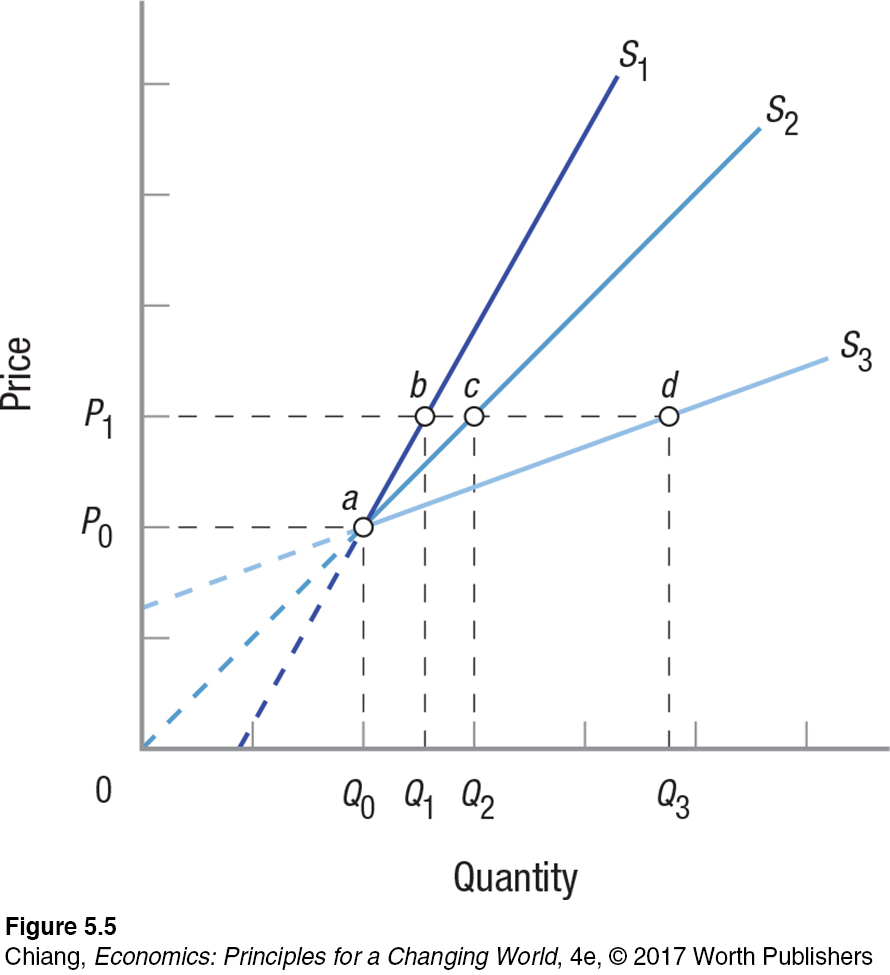
The Market Period The market period is so short that the output and the number of firms in an industry are fixed; firms have no time to change their production levels in response to changes in product price. Consider a raspberry market in the summer. Even if consumers flock to the market, their tastes having shifted in favor of fresh raspberries, farmers can do little to increase the supply of raspberries until two years later. Figure 6 shows a market period supply curve (S_MP) for agricultural products such as raspberries. During the market period, the quantity of product available to the market is fixed at Q₀. If demand changes (shifting from D₀ to D₁), the only impact is on the price of the product. In Figure 6, price moves from P₀ (point e) to P₁ (point a). In summary, if demand grows over the market period, price will rise, and vice versa.

121

Changes in demand over the market period can be devastating for firms selling perishable goods. If demand falls, cantaloupes cannot be kept until demand grows; they must either be sold at a discount or trashed.

The Short Run The short run is defined as a period of time during which plant capacity and the number of firms in the industry cannot change. Firms can, however, change the amount of labor, raw materials, and other variable inputs they employ in the short run to adjust their output to changes in the market. Note that the short run does not imply a specific number of weeks, months, or years. It simply means a period short enough that firms cannot adjust their plant capacity, but long enough for them to hire more labor to increase their production. A restaurant with an outdoor seating area can hire additional staff and open this area in a relatively short timeframe when the weather gets warm, but manufacturing firms usually need more time to hire and train new people for their production lines. Clearly, the time associated with the short run differs depending on the industry.

This also is illustrated in Figure 6. The short-run supply curve, S_SR, is more elastic than the market period curve. If demand grows from D₀ to D₁, output expands from Q₀ to Q₂ and price increases to P₂ as equilibrium moves from point e to point b. Because output can expand in the short run in response to rising demand, the price increase is not as drastic as it was in the market period.

The Long Run Economists define the long run as a period of time long enough for firms to alter their plant capacity and for the number of firms in the industry to change. In the long run, some firms may decide to leave the industry if they think the market will be unfavorable. Alternatively, new firms may enter the market, or existing firms can alter their production capacity. Because all these conceivable changes are possible in the long run, the long-run supply curve is more elastic, as illustrated in Figure 6 by supply curve S_LR. In this case, a rise in demand from D₀ to D₁ gives rise to a small increase in the price of the product, while generating a major increase in output, from Q₀ to Q₃ (point c).

In giving the long-run supply curve S_LR a small but positive slope, we are assuming that an industry’s costs will increase slightly as it increases its output. Firms must compete with other industries to expand production. Wages and other input prices rise in the industry as firms attempt to draw resources away from their immediate competitors and other industries.

122

Some industries may not face added costs as they expand. Fast-food chains, copy centers, and coffee shops seem to be able to reproduce at will without incurring increasing costs. Therefore, their long-run supply curves may be nearly horizontal.

At this point, we have seen how elasticity measures the responsiveness of demand to a change in price and how total revenue is affected by different demand elasticities. We have also seen that supply elasticities are mainly a function of the time needed to adjust to price changes. Next, let’s apply our findings about elasticity to a subject that concerns all of us: taxes.