chiangmicro4e

PERFECT COMPETITION: LONG-RUN ADJUSTMENTS

We have seen that perfectly competitive firms can earn economic profits, normal profits, or losses in the short run because their plant size is fixed, and they cannot exit the industry. We now turn our attention to the long run. In the long run, firms can adjust all factors, even to the point of leaving an industry. And if the industry looks attractive, other firms can enter it in the long run. Why are some industries (such as medical marijuana) thriving, while others (such as photo developing) are declining? The answer is tied to economic profits and losses.

Adjusting to Profits and Losses in the Short Run

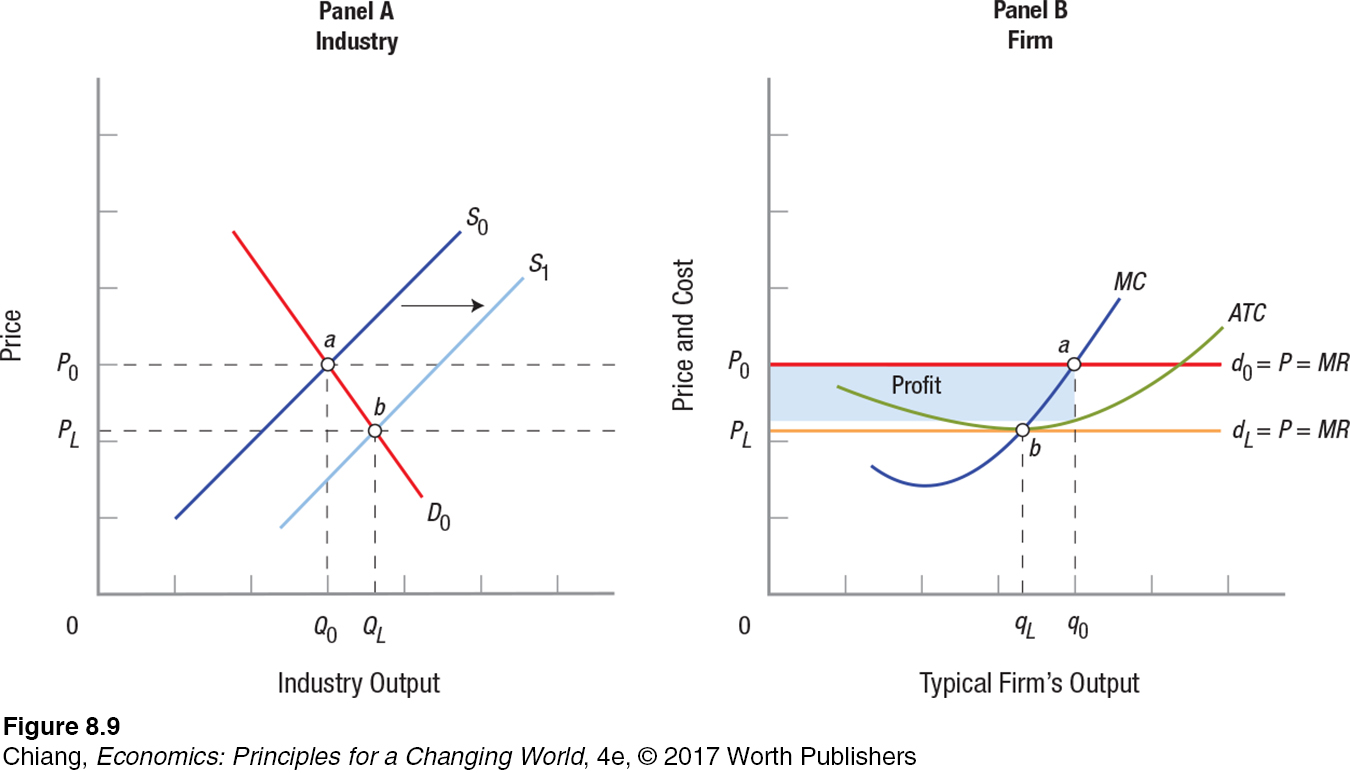
If firms in the industry are earning short-run economic profits, new firms can be expected to enter the industry in the long run, or existing firms may increase the scale of their operations. Figure 9 illustrates one such possible adjustment path when the firms in an industry are earning short-run economic profits. To simplify the discussion, we will assume there are no economies of scale in the long run.

Figure 8.9: FIGURE 9 LONG-RUN ADJUSTMENT WITH SHORT-RUN ECONOMIC PROFITS

Figure 8.9: Panel A shows a market initially in equilibrium at point a. Industry supply and demand equal S₀ and D₀, and equilibrium price is P₀. This equilibrium leads to the short-run economic profits shown in the shaded area in panel B. Short-run economic profits lead other firms to enter the industry, thus raising industry output to Q_L in panel A, while forcing prices down to P_L. The output for individual firms declines as the industry moves to long-run equilibrium at point b. In the long run, firms in perfectly competitive markets can earn only normal profits, as shown by point b in panel B.

207

In panel A, the market is initially in equilibrium at point a, with industry supply and demand equal to S₀ and D₀, and equilibrium price equal to P₀. For the typical firm shown in panel B, this translates into a short-run equilibrium at point a. Notice that, at this price, the firm produces output exceeding the minimum point of the ATC curve. The shaded area represents economic profits.

These economic profits (sometimes called supernormal profits) will attract other firms into the industry. Remember that in a perfectly competitive market, entry and exit are easy in the long run; therefore, many firms decide to get in on the action when they see these profits. As a result, industry supply will shift to the right, to S₁, where equilibrium is at point b, resulting in a new long-run industry price of P_L. For each firm in the industry, output declines to q_L and is just tangent to the minimum point on the ATC curve. Thus, all firms are now earning normal profits and keeping their investors satisfied. There are no pressures at this point for more firms to enter or exit the industry.

Consider the opposite situation—that is, firms in an industry that are incurring economic losses. Figure 10 depicts such a scenario. In panel A, market supply and demand are S₀ and D₀, with equilibrium price at P₀. In panel B, firms suffer economic losses equal to the shaded area. These losses cause some firms to reevaluate their situations and some decide to leave the industry, thus shifting the industry supply curve to S₁ in panel A, generating a new equilibrium price of P_L. This new price is just tangent to the minimum point of the ATC curve in panel B, expanding output for those individual firms remaining in the industry. Firms in the industry are now earning normal profits; therefore, the pressures to leave the industry dissipate.

Figure 8.10: FIGURE 10 LONG-RUN ADJUSTMENT WITH SHORT-RUN LOSSES

Figure 8.10: Panel A shows a market initially in equilibrium at point a. Industry supply and demand equal S₀ and D₀, and equilibrium price is P₀. This equilibrium leads to the short-run economic losses shown in the shaded area in panel B, thus inducing some firms to exit the industry. Industry output contracts to Q_L in panel A, raising prices to P_L and expanding output for the individual firms remaining in the industry, as the industry moves to long-run equilibrium at point b. Again, in the long run, firms in perfectly competitive markets will earn normal profits, as shown by point b in panel B.

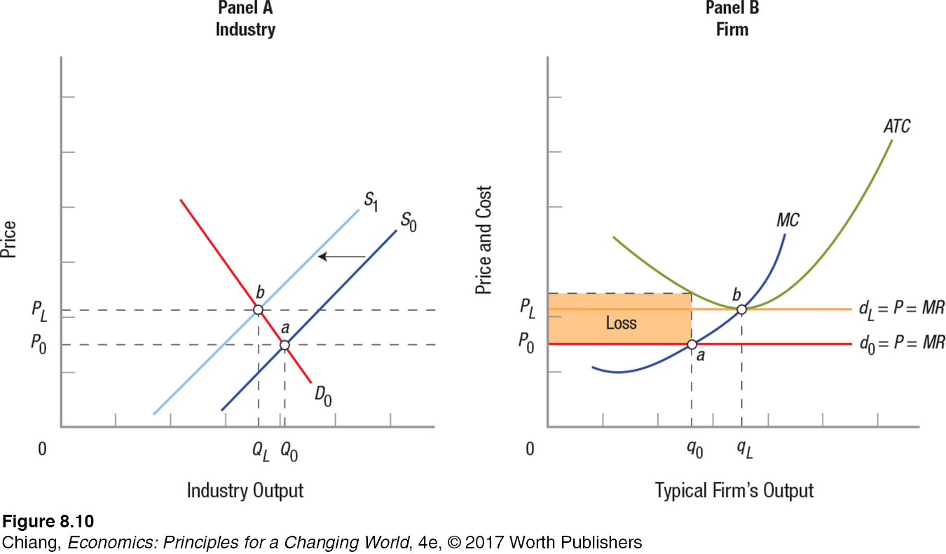
Notice that in Figures 9 and 10, the final equilibrium in the long run is the point at which industry price is just tangent to the minimum point on the ATC curve. At this point, there are no net incentives for firms to enter or leave the industry.

208

If industry price rises above this point, the economic profits being earned will induce other firms to enter the industry; the opposite is true if price falls below this point. A simple way to remember this is with the elimination principle: In a competitive industry in the long run with easy entry and exit, profits are eliminated by firm entry, and losses are eliminated by firm exit.

Competition and the Public Interest

Competitive processes dominate modern life. You and your friends compete for grades, concert tickets, spouses, jobs, and many other benefits. Competitive markets are simply an extension of the competition inherent in daily life. Figure 11 illustrates the long-run equilibrium for a firm in a competitive market. Market price in the long run is P_LR; it is equal to the minimum point on both the short-run average total cost (SRATC) curve and the long-run average total cost (LRATC) curve. At point e, the following is true:

P = MR = MC = SRATC_min = LRATC_min

Figure 8.11: FIGURE 11 LONG-RUN EQUILIBRIUM FOR THE PERFECTLY COMPETITIVE FIRM

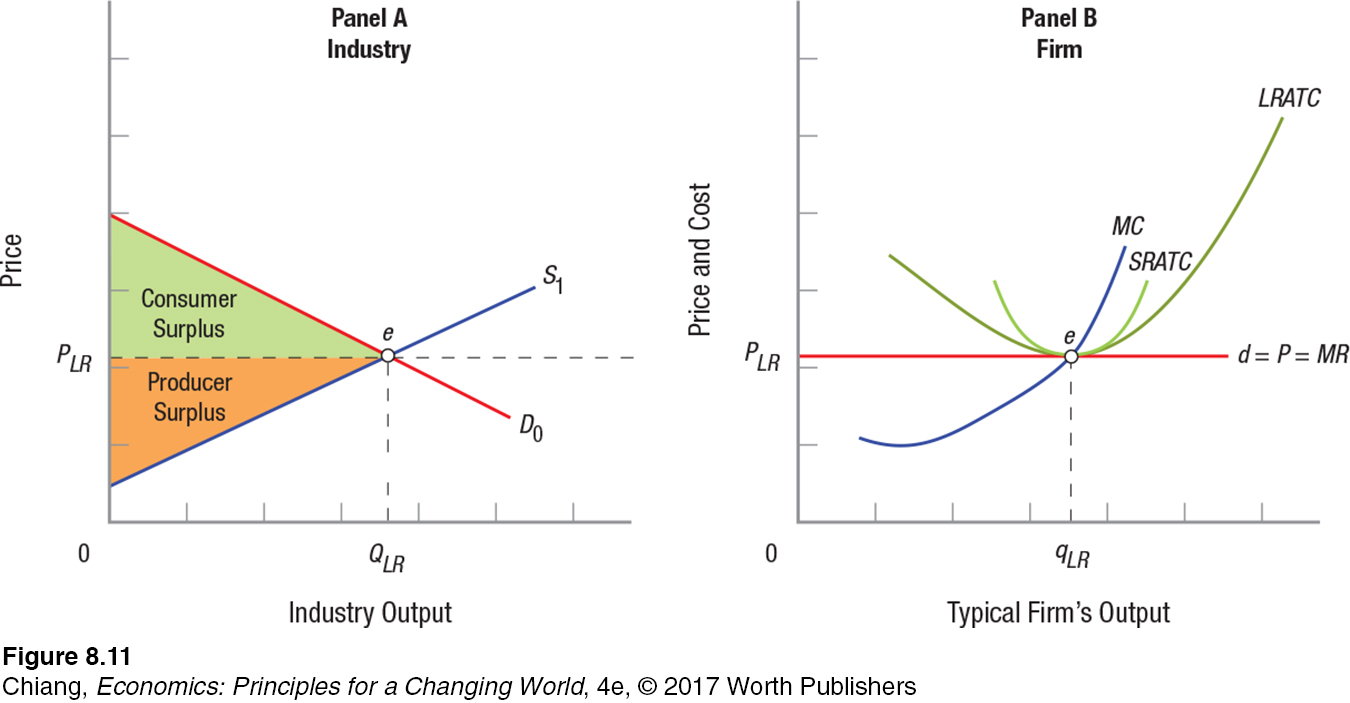
Figure 8.11: Market price in the long run is P_LR, corresponding to the minimum point on the SRATC and LRATC curves. At point e, P = MR = MC = SRATC_min = LRATC_min. This is why economists use perfectly competitive markets as the benchmark when comparing the performance of other market structures. With competition, consumers get just what they want because price reflects their desires, and they get these products at the lowest possible price (LRATC_min). Further, as panel A illustrates, the sum of consumer and producer surplus is maximized. Any reduction in output reduces the sum of consumer and producer surplus.

This equation illustrates why competitive markets are the standard (benchmark) by which all other market structures are evaluated. First, competitive markets exhibit productive efficiency. Products are produced and sold to consumers at their lowest possible opportunity cost. For consumers, this is an excellent situation: They pay no more than minimum production costs plus a profit (a normal profit, to be precise) sufficient to keep producers in business, and consumer surplus shown in panel A is maximized. When we look at monopoly firms in the next chapter, consumers do not get such a good deal.

Second, competitive markets demonstrate allocative efficiency. The price that consumers pay for a given product is equal to marginal cost. Because price represents the value consumers place on a product, and marginal cost represents the opportunity cost to society to produce that product, when these two values are equal, the market is allocating the production of various goods according to consumer wants.

209

Colombian Coffee: The Perils of Existing in a Perfectly Competitive Industry

What aspects of the coffee market make it difficult for Colombian coffee growers to maintain a consistent income every year?

Each day, over 2 billion cups of coffee are consumed globally. Although coffee baristas around the world use their talents to produce the best cup of latte or espresso, the most crucial input remains the coffee bean, which can be produced only in tropical climates with volcanic soil and with the right amount of rain. With an ideal climate, a country can produce billions of pounds of coffee beans, providing income to millions of workers. But what happens when the weather doesn’t cooperate? Farmers in one country, Colombia, can share that experience.

The Image Bank/Getty Images

Colombia has long been one of the largest coffee producers in the world. Although it’s never been the top coffee producer (that award goes to Brazil), Colombian coffee is famous due in large part to Colombia’s ideal climate suited for growing high-quality Arabica beans, along with the marketing of Colombian coffee by the National Federation of Coffee Growers and their famous fictional spokesperson Juan Valdez. Although this may sound like market power, Colombia’s coffee industry faces competition from many countries whose coffee is nearly identical to Colombia’s, making the industry perfectly competitive. Moreover, much like other coffee-producing countries, Colombia’s coffee industry comprises hundreds of thousands of individually owned coffee farms that sell their output to the national federation.

Because the price that individual farmers receive for their coffee is determined by the market, fluctuations in coffee prices can result in a large windfall or a devastating drop in a coffee producer’s household income. Moreover, unpredictable weather patterns and crop diseases, as experienced in recent years, can destroy a harvest altogether. The income risk involved with producing in a perfectly competitive industry such as coffee means that farmers need to prepare for a rainy day, both figuratively and literally.

GO TO TO PRACTICE THE ECONOMIC CONCEPTS IN THIS STORY

210

The flip side of these observations is that if a market falls out of equilibrium, the public interest will suffer. If, for instance, output falls below equilibrium, marginal cost will be less than price. Therefore, consumers place a higher value on that product than it is costing firms to produce. Society would be better off if more of the product were put on the market. Conversely, if output rises above the equilibrium level, marginal cost will exceed price. This excess output costs firms more to produce than the value placed on it by consumers. We would be better off if those resources were used to produce another commodity more highly valued by society.

Long-Run Industry Supply

Recall from an earlier chapter that supply curves tend to be more elastic (flat) over time as businesses have time to adjust their output to changing prices. In addition to responding to market prices, firms also respond to changes in production costs as output changes. Economies or diseconomies of scale determine the shape of the long-run average total cost (LRATC) curve for individual firms. A firm that enjoys significant economies of scale will see its LRATC curve slope down for a wide range of output. Firms facing diseconomies of scale will see their average costs rise as output rises. The nature of these economies and diseconomies of scale determines the size of the competitive firm.

ISSUE

Globalization and “The Box”

When we think of disruptive technologies that radically changed an entire market, we typically think of computers, the Internet, and smartphones. Competitors must adapt to the change or wither away. One disruptive technology we take for granted today, but one that changed our world, is “the box”—the standardized shipping container. Today the vast majority of the world’s deep-sea general cargo is transported in containers.

Before containers, shipping costs added about 25% to the cost of some goods and represented over 10% of U.S. exports. The process was cumbersome; hundreds of longshoremen would remove boxes of all sizes, dimensions, and weight from a ship and load them individually onto trucks (or from trucks to a ship if they were going the other way). This process took a lot of time, was subject to damage and theft, and was costly and inconvenient for business.

Youssouf Cader/Dreamstime.com

In 1955 Malcom McLean, a North Carolina trucking entrepreneur, got the idea to standardize shipping containers. He originally thought he would drive a truck right onto a ship, drop a trailer, and drive off. Realizing that the wheels would consume a lot of space, he soon settled on standard containers that would stack together, but would also load directly onto a truck trailer. Containers are 20 or 40 feet long, 8 feet wide, and 8 or 8½ feet tall. This standardization greatly reduced the costs of handling cargo. McLean bought a small shipping company, called it Sea-Land, and converted some ships to handle the containers. In 1956 he converted an oil tanker and shipped fifty-eight containers from Newark, New Jersey, to Houston, Texas. It took roughly a decade of union bargaining and capital investment by firms for containers to catch on, but the rest is history.

Longshoremen and other port operators thought he was nuts, but as the idea took hold, the West Coast longshoremen went on strike to prevent the introduction of containers. They received some concessions, but containerization was inevitable. Containerization was so cost-effective that it could not be stopped. It set in motion the long-run adjustments we see in competitive markets. Ports that didn’t adjust went out of business, and trucking firms that failed to add containers couldn’t compete. The same was true for oceanic shipping companies.

Much of what we call globalization today can be traced to “the box.” Firms producing products in foreign countries can fill a container, deliver it to a port, and send it directly to the customer or wholesaler in the United States. The efficiency, originally seen by McLean, was that the manufacturer and the customer would be the only ones to load and unload the container, keeping the product safer, more secure, and cutting huge chunks off the cost of shipping. Today, a 40-foot container with 32 tons of cargo shipped from China to the United States costs roughly $5,000 to ship, or 7 cents a pound! This efficient technology has facilitated the expansion of trade worldwide and increased the competitiveness of many industries.

Sources: Based on Mark Levinson, The Box (Princeton, NJ: Princeton University Press), 2006.

211

increasing cost industry An industry that, in the long run, faces higher prices and costs as industry output expands. Industry expansion puts upward pressure on resources (inputs), causing higher costs in the long run.

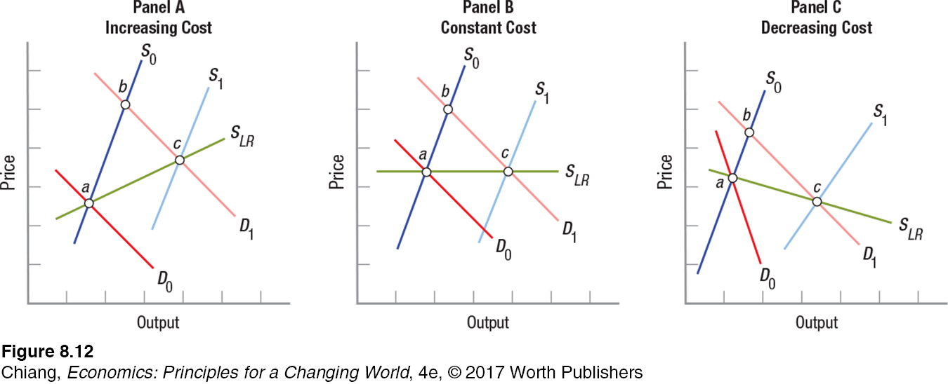
Long-run industry supply is related to the degree to which increases and decreases in industry output influence the prices firms must pay for resources. For example, when all firms in an industry expand or new firms enter the market, this new demand for raw materials and labor may push up the price of some inputs. When this happens, it gives rise to an increasing cost industry in the long run.

To illustrate, panel A of Figure 12 shows two sets of short-run supply and demand curves. Initially, demand and supply are D₀ and S₀, and equilibrium is at point a. Assume demand increases, shifting to D₁. In the short run, price and output will rise to point b. As we have seen earlier, economic profits will result and existing firms will expand or new firms will enter the industry, causing product supply to shift to S₁ in the long run. Note that at the new equilibrium (point c), prices are higher than at the initial equilibrium (point a). This is caused by the upward pressure on the prices of industry inputs, notably raw materials and labor that resulted from industry expansion. Industry output has expanded, but prices and costs are higher. This is an increasing cost industry.

Figure 8.12: FIGURE 12 LONG-RUN INDUSTRY SUPPLY CURVES

Figure 8.12: Panel A shows an increasing cost industry. Demand and supply are initially D₀ and S₀, with equilibrium at point a. When demand increases, price and output rise in the short run to point b. As new firms enter the industry, they drive up the cost of resources. Supply increases in the long run to S₁ and the new equilibrium point c reflects these higher resource costs. In constant cost industries (panel B), firms can expand in the long run without economies or diseconomies; therefore, costs remain constant in the long run. In decreasing cost industries (panel C), expansion leads to external economies and thus to a long-run equilibrium at point c, with lower prices and a higher output than before.

decreasing cost industry An industry that, in the long run, faces lower prices and costs as industry output expands. Some industries enjoy economies of scale as they expand in the long run, typically the result of technological advances.

Alternatively, an industry might enjoy economies of scale as it expands, as suggested by panel C of Figure 12. In this case, price and output initially rise as the short-run equilibrium moves to point b. Eventually, however, this industry expansion leads to lower prices; perhaps suppliers enjoy economies of scale as this industry’s demand for their product increases. The semiconductor industry seems to fit this profile: As the demand for semiconductors has risen over the past few decades, their price has fallen dramatically. In the long run, therefore, a new equilibrium is established at point c, where prices are lower and output is higher than was initially the case. This illustrates what happens in a decreasing cost industry.

constant cost industry An industry that, in the long run, faces roughly the same prices and costs as industry output expands. Some industries can virtually clone their operations in other areas without putting undue pressure on resource prices, resulting in constant operating costs as they expand in the long run.

Finally, some industries seem to expand in the long run without significant change in average cost. These are known as constant cost industries and are shown in panel B in Figure 12. Some fast-food restaurants and retail stores, such as Walmart, seem to be able to clone their operations from market to market without a noticeable rise in costs.

Summing Up

212

This chapter has focused on markets in which there is perfect competition—that is, in which industries contain many sellers and buyers, each so small that they ignore the others’ behavior and sell a homogeneous product. Sellers are assumed to maximize the profits they earn through the sale of their products, and buyers are assumed to maximize the satisfaction they receive from the products they buy. Further, we assume that buyers and sellers have all the information necessary for informed transactions, and that sellers can sell as much of their products as they want at market equilibrium prices.

These assumptions allow us to reach some clear conclusions about how firms operate in competitive markets. In the long run, firms will produce the efficient level of output at which LRATC is minimized, and profits are enough to keep capital in the industry. This output level is efficient because it gives consumers just the goods they want and provides these goods at the lowest possible opportunity costs. Competitive market efficiency represents the benchmark for comparing other market structures.

Competitive markets as we have described them might seem to have such restrictive assumptions that this model only applies to a few industries, such as agriculture, minerals, and lumber. Most businesses you deal with don’t look like the assumptions of these competitive markets. This is true, but most businesses you encounter, such as bars, restaurants, coffee shops, fast-food franchises, cleaners, grocery stores, and shoe and clothing stores, do share some of the characteristics of perfectly competitive markets such as earning normal profits over the long run. In the chapter after next, we examine those markets where consumers see products as differentiated and see how that industry’s behavior is different from a perfectly competitive market.

Because perfect competition is so clearly in the public interest and is the benchmark for comparing other market structures, we can ponder the answer to the following question: Do firms seek the competitive market structure? The answer is: Generally, no. Why? Recall the profit equation. In perfectly competitive markets, firms are price takers. They can achieve economic profits in the short run, but find it almost impossible to have long-run economic profits. Most firms instead want to achieve long-run economic profits. To do so, they must have some ability to control price. In the next chapter, we will see what firms do to achieve this market power.

CHECKPOINT

PERFECT COMPETITION: LONG-RUN ADJUSTMENTS

When perfectly competitive firms are earning short-run economic profits, these profits attract firms into the industry. Supply increases and market price falls until firms are just earning normal profits.
The opposite occurs when firms are making losses in the short run. Losses mean some firms will leave the industry. This reduces supply, thus increasing prices until profits return to normal.
Competitive markets are efficient because products are produced at their lowest possible opportunity cost, and the sum of consumer and producer surplus is at a maximum.
An industry in which prices rise as the industry grows is an increasing cost industry, and increased costs may be caused by rising prices of raw materials or labor as the industry expands.
Decreasing cost industries see their prices fall as the industry expands, possibly due to large economies of scale or rapidly improving technology.
Constant cost industries seem to be able to expand without facing higher or lower costs.

QUESTION: Most of the markets and industries in the world are highly competitive, and presumably most CEOs of businesses know that competition will mean that they will only earn normal profits in the long run. Given this analysis, why do they bother to stay in business, when any economic profits will vanish in the long run?

Answers to the Checkpoint questions can be found at the end of this chapter.

All businesses are looking for the “next new thing” that will generate economic profits and propel them to monopoly status. Even normal profits are not trivial. Remember, normal profits are sufficient to keep investors happy in the long run. When firms do find the right innovation, such as the iPad, Windows operating system, or a blockbuster drug, the short-run returns can be tremendous.