11.1 Introduction to Repeated-Measures ANOVA
In this chapter, we learn about within-subjects ANOVA, commonly called repeated-measures ANOVA. Repeated-measures ANOVA is an extension of the paired-samples t test. The paired-samples t test can only be used when comparing the means of two dependent samples. But, a repeated-measures ANOVA can be used when there are two or more dependent samples.
There are many different types of experiments that use repeated measures. What they have in common is a connection between the cases in one cell and the cases in the other cells. Repeated measures may involve:
The same cases measured at multiple points of time. For example, to examine how weight changes over college, a group of first-year college students might be weighed at the start and the end of each of the four years of college.
382
The same cases measured under multiple conditions. For example, to examine how alcohol affects one’s ability to walk a straight line, 21-year-olds might be asked to walk a straight line before drinking anything, after drinking a placebo beer, after drinking one beer, after two, after four, and after six.
Different cases, matched so that they are similar in some dimension(s). For example, a researcher comparing murder rates for cities with high, medium, and low numbers of sunny days per year might be concerned that population density and poverty level could affect the results. To account for these other factors, he could group cities with the same populations and unemployment rates into sets of three: one with a high number of sunshine days, one low on the number of sunshine days, and one in the middle.
In all these examples of dependent samples, we’re looking at differences within the same subjects (or matched subjects) over time or across conditions (the treatment). Thus, it is important to make sure that the subjects are arrayed in the same order from cell to cell to cell. If a participant’s data point is listed first in one cell, then it should be first in the other cells.
The beauty of analysis of variance is that it partitions the variability in the dependent variable into the components that account for the variability. Between-subjects, one-way ANOVA, covered in the last chapter, distinguishes variability due to how the groups are treated (between-group variability) from variability due to individual differences among subjects (within-group variability). With between-subjects ANOVA, it doesn’t matter how subjects in a cell are arrayed. In our example, the three rats that ran the maze to reach low-calorie food ran it in 30, 31, and 32 seconds. And that is how the data showed up in the first cell of Table 10.3. But, the data could just as easily have been listed as 31, 32, and 30 or as 31, 30, and 32. These cases are independent of each other. No matter the order that the results are listed, the results of the between-subjects ANOVA will be the same. This is not true of repeated-measures ANOVA. Because the samples in repeated-measures ANOVA are dependent samples, the order in which they are arranged matters very much. Changing the order, unless it is changed consistently in all cells, will change the outcome.
In repeated-measures ANOVA, the levels of the independent variable, for example, the different times or conditions, make up the columns and the subjects make up the rows. By having each subject on a row by itself, subjects can be treated as a second explanatory variable, as a second factor. Treating subjects as a factor allows repeated-measures ANOVA to measure—to account for—variability due to them. By partitioning out this variability, repeated-measures ANOVA obtains a purer measure of the effect of treatment and is a more statistically powerful test than is between-subjects ANOVA. What does it mean to be a statistically more powerful test? It means that this test gives us a greater likelihood of being able to reject the null hypothesis.
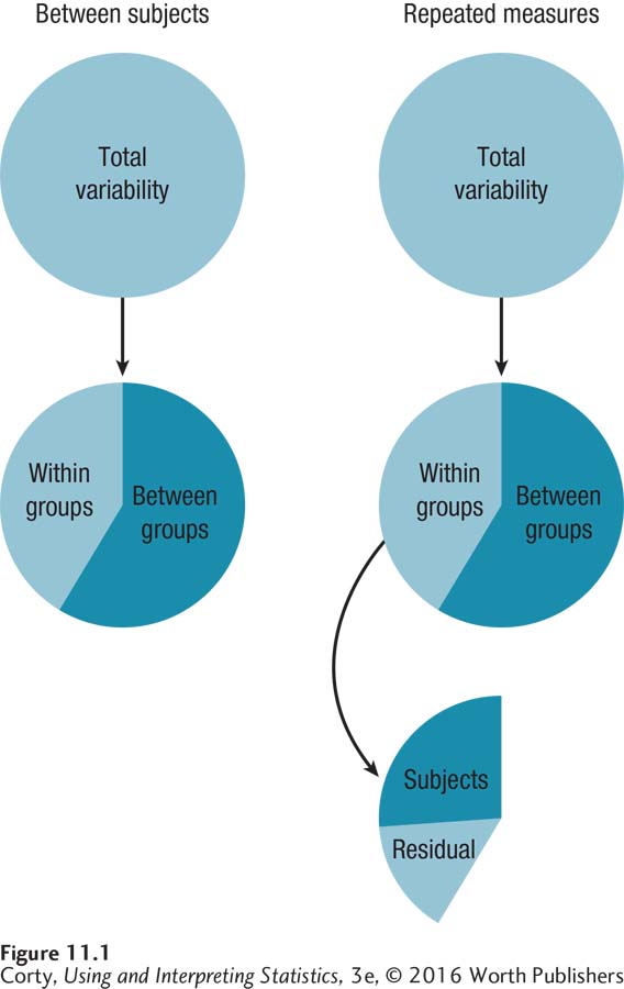
Figure 11.1 shows the similarities and differences between the sources of variability for between-subjects and repeated-measures ANOVA. With between-subjects ANOVA, total variability is partitioned into between and within. For repeated-measures ANOVA, total variability is also partitioned into between and within. But, within-group variability is then broken down further. First, variability due to subjects is removed. Then, the variability left over, labeled “residual,” is used as the denominator in the F ratio.
383
The statistical power of repeated-measures ANOVA comes from the fact that it partitions out the variability due to subjects. Between-subjects ANOVA divides between-group variability by within-group variability to find the F ratio. Repeated-measures ANOVA calculates between-group variability the same way, so it will have the same numerator for the F ratio. But the denominator, which has variability due to subjects removed, will be smaller. This means that the F ratio will be larger—meaning it is more likely to fall in the rare zone, and therefore more likely to result in a rejection of the null hypothesis than for between-subjects, one-way ANOVA.
To see what this means, let’s analyze the same set of data two ways—one way that doesn’t partition out the subject variability and one that does. Let’s compare two neighboring cities, Erie, PA, and Cleveland, OH, to see if they differ in how hot they get. From weather archives, we have obtained the average high temperature for each city for each month of the year. The data are seen in Figure 11.2. Two things are readily apparent in this graph:
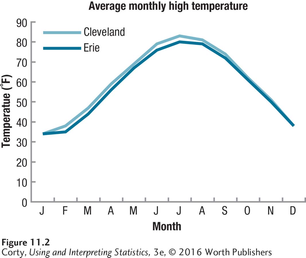
The high temperatures in the two cities are very similar to each other.
Both cities share a strong seasonal trend to temperature—it is hottest in the summer and coldest in the winter.
384
The paired-samples t test is appropriate to use to see if there is a statistically significant difference in temperature between the two cities. The t value turns out to be 5.38 and the difference between the two cities is a statistically significant one—Cleveland with a mean high temperature of 59.6°F is statistically significantly hotter than Erie with a mean of 57.7°F. A difference of 1.9°F doesn’t sound like much, but it is enough to be statistically significant when analyzed with a paired-samples t test.
The reasonable next question to ask is what the size of the effect is. How much of the variability in the dependent variable of temperature is explained by the grouping variable of city? Judging by Figure 11.2, it shouldn’t be much, right? Well, be surprised—72% of the variability in temperature is accounted for by city status! (This book does NOT advocate calculating either d or r2 for a paired-samples t test. In this one instance, however, and just for this one example, I calculated r2.)
An r2 of 72% is a huge effect, a whopping effect. Look at Figure 11.2 again. How can we account for the variability in temperature? Is there more variability in temperature due to differences between the cities each month or is there more variability in temperature due to changes from month to month? Clearly, more variability exists from month to month, which is due to individual differences among our cases, which are months. Regardless of city, months like July and August differ by 40 to 50 degrees F from months like January and February.
Does it make sense that the variability in temperature accounted for by the between-groups factor, city, is 72%? No! And it can’t be so. If we just agreed that more of the variability in Figure 11.2 is due to the within-group factor (month) than the between-group factor, and the between-group factor accounted for 72% of the variability, then the within-group factor must explain at least 73% of the variability. That’s impossible—we have just accounted for at least 145% of the variability!
So, what is going on? Because a paired-samples t test doesn’t partition out the variability due to subjects, it mixes in variability due to individual differences with variability due to the grouping variable when calculating r2. Thus, r2 is an overestimate of the percentage of variability due to the grouping variable and should not be used with paired-samples t tests. The same is true for Cohen’s d for a paired-samples t test—it also overestimates the size of the effect.
How much of the variability in temperature is really due to the grouping variable of city? To answer that, we need a repeated-measures ANOVA, which treats variability due to the independent variable and that due to the subjects separately. ANOVA, which can be used when comparing two or more means, can be used in place of a t test. As we are about to see, there is a distinct advantage to using a repeated-measures ANOVA over a paired-samples t test.
When these temperature data are analyzed with a repeated-measures ANOVA, the difference between the mean temperatures due to location is still a statistically significant one. But now, because the variance due to subjects has been removed, the effect size will be a purer measure of the effect of the independent variable. By removing individual subject variability, the explanatory power of the city where the measurement was taken is reduced from 72% to1%. Yes, 1%. Look at Figure 11.2 again. Doesn’t a measure of 1% of the variability due to location reflect reality a lot better than 72%? If you are comparing the means of two dependent samples, use repeated-measures ANOVA, not a paired-samples t test.
385
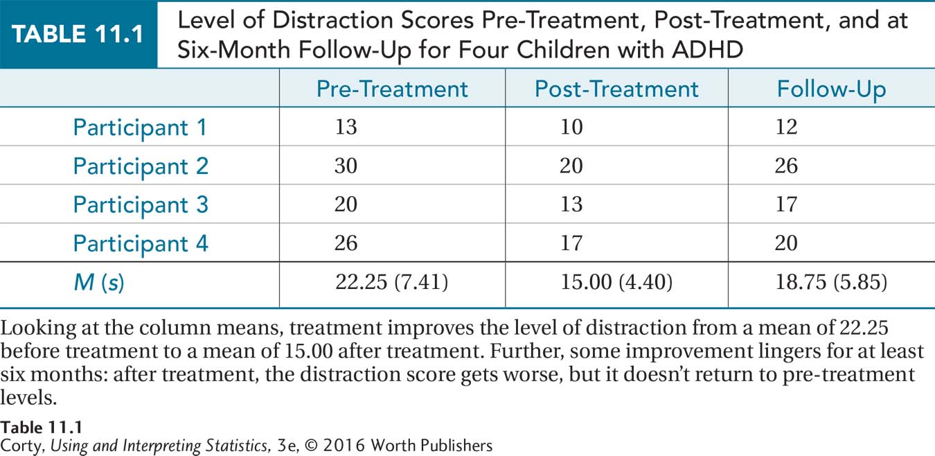
We’ll use the following example throughout the chapter to learn how to complete a repeated-measures ANOVA. Imagine that Dr. King wanted to determine if a new treatment for ADHD was effective. He took four children with ADHD and measured their level of distraction on an interval-level scale where higher scores mean a higher level of distraction. Next, each child received individual behavior therapy for three months, after which the child’s level of distraction was assessed again. Finally, to determine if the effects of treatment are long-lasting, each child had his or her level of distraction measured again six months later.
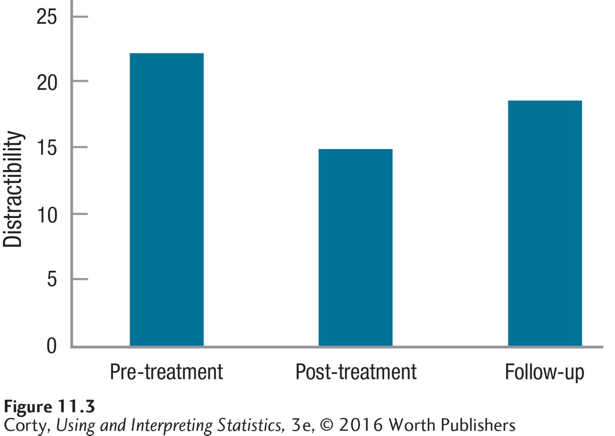
Table 11.1 contains the data, each case in its own row and each phase of treatment in a separate column. The effects of treatment are found in the column means. Figure 11.3 shows that the mean level of distraction is highest before the treatment starts, lowest at the end of treatment, and somewhere in the middle at follow-up. This suggests that treatment has an effect on reducing distraction and that the effect lingers, though in a weakened form, for six months. Of course, Dr. King needs to do a statistical test to determine if the treatment effect is statistically significant or if the differences can be accounted for by sampling error.
386
The differences between rows are due to individual differences, uncontrolled characteristics that vary from case to case. For example, case 1 has the lowest level of distraction pre-treatment. This could be due to the participant’s having a less severe form of ADHD, having eaten a good breakfast on the day of the test, having been taught by a teacher who stressed the skills on the test, or a whole host of other uncontrolled factors.
To reiterate the message of this introduction, the effect of individual differences is intertwined with the effect of treatment. Is the first case’s low score at the end of treatment due to the effect of treatment or due to individual differences like a less severe form of ADHD? One-way, repeated-measures ANOVA is statistically powerful because it divides the variability in scores into these two factors. Repeated-measures ANOVA determines (1) how much variability is due to the column effect (the effect of treatment), and (2) how much variability is due to the row effect (individual differences). Let’s see it in action in the next section.
Practice Problems 11.1
Review Your Knowledge
11.01 When is repeated-measures ANOVA used?
11.02 Into what two factors does one-way, repeated-measures ANOVA divide variability in a set of scores?
11.03 When comparing the means of two dependent samples, what test should be used? Why?