CHAPTER EXERCISES
Answers to the odd-numbered exercises appear in Appendix B.
Review Your Knowledge
11.01 Between-subjects, one-way ANOVA extends the ____ to situations in which there are more than two independent samples.
11.02 Within-subjects, one-way ANOVA is like between-subjects, one-way ANOVA but is for ____ samples.
411
11.03 ____ ANOVA is the common name for within-subjects, one-way ANOVA.
11.04 Repeated-measures ANOVA is used to compare the ____ of ____ or more dependent samples.
11.05 The data used in repeated-measures ANOVA are arranged with cases on ____ and levels of the explanatory variable in ____.
11.06 In repeated-measures ANOVA, the cases should be in the ____ order in each cell.
11.07 Because a repeated-measures ANOVA is more ______ than a between-subjects, one-way ANOVA, there is a ____ likelihood of being able to reject the null hypothesis.
11.08 What is called the between-groups effect in between-subjects, one-way ANOVA is called the _____ effect in repeated-measures ANOVA.
11.09 Because variability due to subjects is removed from within-groups variability in repeated-measures ANOVA, the numerator/denominator of the F ratio is smaller than it is in between-subjects, one-way ANOVA.
11.10 If r2 is calculated for a paired-samples t test, it will over / underestimate the effect size.
11.11 When comparing the means of two dependent samples, the author advocates using ____, not ____.
11.12 The random samples assumption says that the samples in a repeated-measures ANOVA are ____ samples from the population to which one wishes to generalize the results.
11.13 The random samples assumption is ____ to violation.
11.14 If cases within a sample influence each other’s scores on the dependent variable, then the ____ assumption is ____.
11.15 It is often assumed that the dependent variable, if it is of a psychological attribute, is ____ in the ____.
11.16 “All population means are equal.” This is the ____ hypothesis.
11.17 µ1 ≠ µ2 ≠ µ3 is / is not an accurate statement of the alternative hypothesis.
11.18 The abbreviation for the critical value of F is ____.
11.19 The null hypothesis is rejected if F is ____ the critical value of F.
11.20 The null hypothesis is not rejected if F is ____ the critical value of F.
11.21 If the results are called statistically significant, then the null hypothesis was / was not rejected.
11.22 If the conclusion of a repeated-measures ANOVA is that there is no evidence of a difference among population means, then the null hypothesis was / was not rejected.
11.23 If one was forced to accept the alternative hypothesis, then the null hypothesis was / was not rejected.
11.24 Values of Fcv depend on the numerator and denominator ____.
11.25 df ____ are the numerator degrees of freedom for a one-way, repeated-measures ANOVA and df ____ are the denominator degrees of freedom.
11.26 df ____ and df ____ are not needed to find Fcv for a one-way, repeated-measures ANOVA.
11.27 To apply Equation 11.1 to calculate all 4 degrees of freedom, one needs to know ____, ____, and ____.
11.28 To calculate N, one multiplies together ____ and ____.
11.29 If one adds together dfSubjects, dfTreatment, and dfResidual, this equals ____.
11.30 One-way, repeated-measures ANOVA divides dfTotal into subcomponents for two different sources of ____.
11.31 The effect of individual differences in repeated-measures ANOVA is called the effect of ____ in the ANOVA summary table.
11.32 After dfSubjects and dfTreatment are removed from dfTotal, what is left is called ____.
412
11.33 If the observed value of F falls in the ____ zone of the sampling distribution, the null hypothesis is rejected.
11.34 If F falls on the line that separates the rare zone from the common zone, the null hypothesis is / is not rejected.
11.35 The first column in an ANOVA summary table lists the sources of ____.
11.36 If one knows SSSubjects, SSTreatment, and SSResidual, one can calculate SS____.
11.37 To calculate a mean square, one divides a ____ by its ____.
11.38 The only mean squares one needs to calculate for a one-way, repeated-measures ANOVA are MS ____ and MS ____.
11.39 The F ratio for one-way, repeated-measures ANOVA is ____ divided by ____.
11.40 The first question to be addressed in an interpretation of a one-way, repeated-measures ANOVA is ____.
11.41 By implementing the ____ from Step 4, one can determine if the results of a statistical test are statistically significant.
11.42 If one knows that the null hypothesis for a one-way, repeated-measures ANOVA was rejected, one does / does not know which pairs of sample means had statistically significant differences.
11.43 Results were reported in APA format as F(2, 12) = 7.89, p < .05. The null hypothesis was / was not rejected.
11.44 Results were reported in APA format as F(2, 22) = 0.89, p > .01. The alpha level was ____.
11.45 If the null hypothesis is not rejected, one should / should not calculate an effect size.
11.46 Eta squared provides information about the size of the ____.
11.47 A researcher ends up suggesting replication of study with a larger sample size. The null hypothesis probably was / was not rejected.
11.48 If a researcher suggests replication with a larger sample size, then he or she is probably worried about Type ____ error.
11.49 The effect size used with one-way, repeated-measures ANOVA is ____.
11.50 Eta squared tells the percentage of variability in the ____ variable that is explained by the ____ variable.
11.51 Eta squared, like ____, ranges from 0% to100%.
11.52 The closer eta squared is to ____%, the bigger the effect.
11.53 If the treatment effect explained 10% of the variability in a set of scores, Cohen would consider this a ____ effect.
11.54 The ____ is a post-hoc test for use with one-way, repeated-measures ANOVA.
11.55 Post-hoc tests for ANOVA should only be calculated when the null hypothesis is ____.
11.56 To calculate an HSD value, one needs to find a ____ value in Appendix Table 5.
11.57 If a pair of sample means differ by less than the HSD value, the difference is considered ____ significant.
11.58 If a difference in a post-hoc test is statistically significant, the two sample means can be used to determine the ____ of the difference for the two population means.
Apply Your Knowledge
Selecting the appropriate statistical test.
(For 11.59–11.62, select from the single-sample z test; single-sample t test; independent-samples t test; paired-samples t test; between-subjects, one-way ANOVA; and one-way, repeated-measures ANOVA.)
11.59 People who traveled between Philadelphia and New York City by different vehicles (train, car, bus, or plane) were surveyed to see how pleasant the experience had been. Pleasantness was measured on an interval scale. What statistical test should be used to analyze these data to see if different modes of travel were associated with different mean levels of pleasantness?
413
11.60 First-year college students were surveyed about how much they liked their roommates (a) within five minutes of meeting them, (b) after the first week of classes, and (c) at the end of the semester. An interval measure of liking was used. What statistical test should be used to see if the mean degree of liking changed over the course of the semester?
11.61 When making purchases with cash, some people drop their pennies in the “penny cup” next to the cash register and some don’t. A social psychologist wondered if those who did were more altruistic. She obtained a sample of people who dropped their pennies into penny cups and a sample who didn’t. To each person, she administered an interval-level measure of altruism. What statistical test should she use to see if the groups differ on the mean level of altruism?
11.62 A recreational therapist knows the U.S. population mean and standard deviation for scores on an interval-level risk-taking scale. She obtains a random sample of people who enjoy riding roller coasters at amusement parks and has them complete the risk-taking scale. What statistical test should she use to see if roller coaster riders differ in the mean level of sensation-seeking from the general population?
Checking the assumptions for a one-way, repeated-measures ANOVA and deciding if it is OK to proceed with the test
11.63 The dean of retention at a college wanted to find out if academic problems or social problems caused students to drop out at her college. She took a random sample of first-year students at her college and, on the basis of SAT scores, matched them into groups of three. One member of each group was then randomly assigned to be in (a) the control group, (b) the academic enhancement group, or (c) the social enhancement group. Nothing was done to the control participants. The academic enhancement participants met together as a group 10 times over the course of the semester, to cover study skills, time management, test anxiety, and so on. The social enhancement participants also met together as a group 10 times over the course of the semester, though the focus was on social skills, dating, alcohol safety, and the like. At the end of the semester, she compared the three group means on the interval-level Adjustment to College Inventory.
For each of the three assumptions for a one-way, repeated-measures ANOVA, determine if it was violated.
Decide if the dean can proceed with the one-way, repeated-measures ANOVA.
11.64 A clinical psychologist wanted to compare three treatments for generalized anxiety disorder (GAD). She put an ad in the local paper to find people with GAD. She matched them into groups of three, based on severity of symptoms, and randomly assigned each of the matched cases to one of the three treatments. Treatment was administered individually. Outcome was assessed at the end of treatment using an interval-level measure of generalized anxiety.
For each of the three assumptions for a one-way, repeated-measures ANOVA, determine if it was violated.
Decide if the psychologist can proceed with the one-way, repeated-measures ANOVA.
Stating the hypotheses for a one-way, repeated-measures ANOVA
11.65
What is the null hypothesis for a one-way, repeated-measures ANOVA?
What is the alternative hypothesis for a one-way, repeated-measures ANOVA?
11.66
What is the null hypothesis for Exercise 11.64?
What is the alternative hypothesis for Exercise 11.64?
Calculating degrees of freedom for one-way, repeated-measures ANOVA
11.67 If k = 3, n = 8, and N = 24, what are dfSubjects, dfTreatment, dfResidual, and dfTotal?
11.68 If k = 5, n = 20, and N = 100, what are dfSubjects, dfTreatment, dfResidual, and dfTotal?
11.69 If k = 4 and n = 15, what are dfSubjects, dfTreatment, dfResidual, and dfTotal?
414
11.70 If k = 3 and n = 30, what are dfSubjects, dfTreatment, dfResidual, and dfTotal?
Setting the decision rule for one-way, repeated- measures ANOVA (assume α = .05)
11.71 Given dfTreatment = 2 and dfResidual = 10, (a) what is Fcv? (b) Draw the sampling distribution of F, being sure to label the common zone, the rare zone, and Fcv.
11.72 Given dfTreatment = 3 and dfResidual = 36, (a) what is Fcv? (b) Draw the sampling distribution of F, being sure to label the common zone, the rare zone, and Fcv.
11.73 If dfTreatment = 3 and dfResidual = 15, state the decision rule.
11.74 If dfTreatment = 2 and dfResidual = 76, state the decision rule.
Calculating F
11.75 Given the following, complete an ANOVA summary table for a one-way, repeated-measures ANOVA: dfSubjects = 11, dfTreatment = 2, dfResidual = 22, dfTotal = 35, SSSubjects = 137.50, SSTreatment = 48.48, SSResidual = 115.50, and SSTotal = 301.48.
11.76 Given the following, complete an ANOVA summary table for a one-way, repeated-measures ANOVA: dfSubjects = 19, dfTreatment = 3, dfResidual = 57, dfTotal = 79, SSSubjects = 101.27, SSTreatment = 99.81, SSResidual = 957.48. and SSTotal = 1,158.56.
Rejecting the null hypothesis?
11.77 If Fcv = 3.259 and F = 3.259, was H0 rejected?
11.78 If Fcv = 2.310 and F = 1.96, was H0 rejected?
11.79 Using the information in this ANOVA summary table, determine if the null hypothesis is rejected if alpha is set at .05:
| Source of Variability | Sum of Squares | Degrees of Freedom | Mean Square | F ratio |
| Subjects | 5.00 | 20 | ||
| Treatment | 5.00 | 2 | 2.50 | 5.00 |
| Residual | 20.00 | 40 | 0.50 | |
| Total | 30.00 | 62 |
11.80 Using the information in this summary table, determine if the null hypothesis is rejected if alpha is set at .05:
| Source of Variability | Sum of Squares | Degrees of Freedom | Mean Square | F ratio |
| Subjects | 12.50 | 17 | ||
| Treatment | 5.00 | 3 | 1.67 | 1.78 |
| Residual | 48.00 | 51 | 0.94 | |
| Total | 65.50 | 71 |
Writing results in APA format
11.81 Given α = .05, dfTreatment = 5, dfResidual = 45, F = 7.84, and Fcv = 2.579, (a) write the results in APA format, and (b) state if the results are statistically significant or not.
11.82 Given α = .05, dfTreatment = 3, dfResidual = 24, F = 2.76, and Fcv = 3.009, (a) write the results in APA format, and (b) state if the results are statistically significant or not.
11.83 Given α = .05 and the information in this summary table, (a) write the results in APA format, and (b) state if the results are statistically significant or not:
| Source of Variability | Sum of Squares | Degrees of Freedom | Mean Square | F ratio |
| Subjects | 88.00 | 9 | ||
| Treatment | 60.00 | 2 | 30.00 | 11.24 |
| Residual | 48.00 | 18 | 2.67 | |
| Total | 196.00 | 29 |
11.84 Given α = .05 and the information in this summary table, (a) write the results in APA format, and (b) state if the results are statistically significant or not:
| Source of Variability | Sum of Squares | Degrees of Freedom | Mean Square | F ratio |
| Subjects | 120.00 | 21 | ||
| Treatment | 32.00 | 2 | 16.00 | 1.00 |
| Residual | 674.00 | 42 | 16.05 | |
| Total | 826.00 | 65 |
415
Interpreting results
11.85 Given the results of a one-way, repeated-measures ANOVA in APA format, F(2, 40) = 1.52, p > .05, interpret them based only on this.
11.86 Given the results of a one-way, repeated-measures ANOVA in APA format, F(3, 36) = 12.56, p < .05, interpret them based only on this.
Calculating effect size
11.87
Given SSTreatment = 9.89 and SSTotal = 86.98, what is η2?
Classify it as small, medium, or large.
11.88
Given SSTreatment = 45.55 and SSTotal = 1,893.44, what is η2?
Classify it as small, medium, or large.
11.89
Given the information in this summary table, what is η2?
Classify it as small, medium, or large.
| Source of Variability | Sum of Squares | Degrees of Freedom | Mean Square | F ratio |
| Subjects | 76.00 | 14 | ||
| Treatment | 46.00 | 2 | 23.00 | 3.01 |
| Residual | 214.00 | 28 | 7.64 | |
| Total | 336.00 | 44 |
11.90
Given the information in this summary table, what is η2?
Classify it as small, medium, or large.
| Source of Variability | Sum of Squares | Degrees of Freedom | Mean Square | F ratio |
| Subjects | 233.00 | 16 | ||
| Treatment | 111.00 | 2 | 55.50 | 5.35 |
| Residual | 332.00 | 32 | 10.38 | |
| Total | 676.00 | 50 |
Worrying about Type II error
11.91 If the results of a one-way, repeated-measures ANOVA are F(2, 42) = 0.63, p > .05 and if η2 = 2.12%, (a) how worried should the researcher be about having made a Type II error? (b) Should he or she recommend replication with a larger sample size?
11.92 If the results of a one-way, repeated-measures ANOVA are F(2, 58) = 3.00, p > .05 and if η2 = 8.11%, (a) how worried should the researcher be about having made a Type II error? (b) Should he or she recommend replication with a larger sample size?
Finding q
11.93 If k = 3 and dfResidual = 16, what is q if α = .01?
11.94 If k = 4 and dfResidual = 87, what is q if α = .05?
Calculating HSD
11.95 If q = 2.90, MSResidual = 12.27, and n = 8, what is HSD?
11.96 If q = 3.70, MSResidual = 122.98, and n = 30, what is HSD?
Interpreting HSD
11.97 If M1 = 12.83, M2 = 14.98, M3 = 8.22, and HSD = 3.78, (a) determine for each possible pair of means if the difference is statistically significant, and (b) comment on the direction of the difference for the populations.
11.98 If M1 = 115.54, M2 = 98.98, M3 = 118.22, and HSD = 14.78, (a) determine for each possible pair of means if the difference is statistically significant, and (b) comment on the direction of the difference for the populations.
Writing a complete interpretation
11.99 Researchers from PETA and NIH collaborated on a study to examine the effect, on rats, of being reared in laboratory settings. Sets of 3 rats from 8 litters were randomly assigned to three conditions: (1) being reared in a standard laboratory setting, (2) being reared in an enriched laboratory setting, and (3) being reared in a setting that mimics the wild (e.g., the rats have to forage for their own food; food is occasionally sparse and of poor quality). When the rats reached adulthood, they were given a series of behavioral tasks from which their rat IQ (RIQ) scores were calculated. RIQ scores are interval-level and are scored like human IQ scores. The three means were 95.00 (normal lab), 108.00 (enriched lab), and 94.00 (mimicked wild). No nonrobust assumptions were violated and a one-way, repeated-measures ANOVA was completed with α = .05. The results are shown below. Fcv was 3.739, η2 was calculated as 37.14%, and HSD was found to be 9.32. Write a four-point interpretation.
416
| Source of Variability | Sum of Squares | Degrees of Freedom | Mean Square | F ratio |
| Subjects | 941.33 | 7 | ||
| Treatment | 976.00 | 2 | 488.00 | 9.61 |
| Residual | 710.67 | 14 | 50.76 | |
| Total | 2,628.00 | 23 |
11.100 A women’s studies professor was curious about the long-term effect, on men, of taking a women’s studies class. She thought that it would make them more open-minded and less sexist. She obtained a random sample of 10 first-year male students at her university and assigned them to take Introduction to Women’s Studies. She administered a scale that measures sexist beliefs before the class started, again at the end of the semester, and again 10 years later. The scale measures at the interval level and has a mean of 50, with a standard deviation of 10. Scores above 50 indicate a person has more sexist beliefs than average; scores below 50 indicate a person has fewer sexist beliefs than average. Here are the mean scores for her 10 participants: 54.00 (pre-class), 46.00 (post-class), 38.00 (10 years later). No assumptions were violated and a one-way, repeated-measures ANOVA, with the alpha set at .05, was completed. Results are shown below. Fcv = 3.555, η2 = 33.21%, HSD = 5.10. Given this information, complete a four-point interpretation.
| Source of Variability | Sum of Squares | Degrees of Freedom | Mean Square | F ratio |
| Subjects | 2,215.33 | 9 | ||
| Treatment | 1,280.00 | 2 | 640.00 | 32.11 |
| Residual | 358.67 | 18 | 19.93 | |
| Total | 3,854.00 | 29 |
Completing all six steps of hypothesis testing
11.101 A psychologist studying addictions investigated the effectiveness of three different treatments for alcoholism on the number of strong urges to drink alcohol that were experienced at the end of treatment. He compared three treatments: (1) Alcoholics Anonymous, (2) individual psychotherapy, and (3) a medication that is supposed to reduce urges. He matched 30 alcoholics into groups of three based on the severity of their addiction and then randomly assigned them to the three different treatments. (Each person assigned to Alcoholics Anonymous attended a different group.) At the end of treatment, he had the participants keep a diary of how many strong urges to drink alcohol they experienced each day. Here are the results:
| Alcoholics Anonymous | Individual Psychotherapy | Medication | |
| M | 8.00 | 6.00 | 6.00 |
| s | 5.42 | 4.52 | 4.37 |
Given SSSubjects = 532.00, SSTreatment = 26.67, SSResidual = 88.00, and SSTotal = 646.67, complete the appropriate statistical test and interpret the results. (Don’t forget to follow all six steps of the hypothesis test.)
11.102 A psychologist teaching introductory psychology wanted to demonstrate the effects of mere exposure on liking. On the first day of class, each of her 20 students went to a private booth to view a very abstract piece of modern art. Each was asked to rate how much he or she liked it on a scale ranging from −10 (extremely dislike) to +10 (extremely like). She followed the same procedure once a week for the rest of the semester. At the middle, and again at the end, of the semester, she had the students individually rate their liking of the picture. Here are the results:
| First Class | Mid-Semester | Last Class | |
| M | −6.30 | −2.40 | 1.70 |
| s | 2.85 | 2.35 | 1.75 |
417
Given SSSubjects = 176.67, SSTreatment = 640.13, SSResidual = 140.53, and SSTotal = 957.33, complete the appropriate statistical test and interpret the results. (Don’t forget to follow all six steps of the hypothesis test.)
Expand Your Knowledge
11.103 If the results of a one-way, repeated-measures ANOVA are F(3, 45) = 12.56, p < .05, what is N?
11.104 Is it possible, in a one-way, repeated-measures ANOVA, for dfTreatment to be 2 and dfResidual to be 75?
11.105 If the results of a one-way, repeated-measures ANOVA are F(3, 45) = 12.50, p < .05, and η2 = 28.30, how concerned should one be about Type II error?
11.106 A group of students had their IQs measured at the start, middle, and end of a school year. The three means, respectively, were 125.5, 127.5, and 130.5. A one-way, repeated-measures ANOVA was used to analyze the data and the results were F(2, 18) = 0.12, p > .05. Use the summary table below to conduct post-hoc tests as appropriate.
| Source of Variability | Sum of Squares | Degrees of Freedom | Mean Square | F ratio |
| Subjects | 4,917.50 | 9 | ||
| Treatment | 126.67 | 2 | 63.34 | 0.12 |
| Residual | 9,590.00 | 18 | 532.78 | |
| Total | 14,634.17 | 29 |
11.107 Which HSD value will be larger: one for α = .01 or one for .05? Why?
SPSS
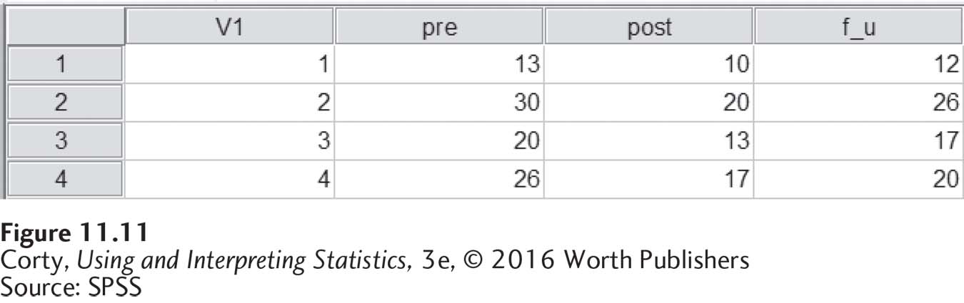
Data entry in SPSS for one-way, repeated-measures ANOVA is similar to data entry for a paired-samples t test—each case has a row to itself and the repeated measures each have a column. Figure 11.11 shows the data from the ADHD/level of distraction study in the SPSS Data Editor.
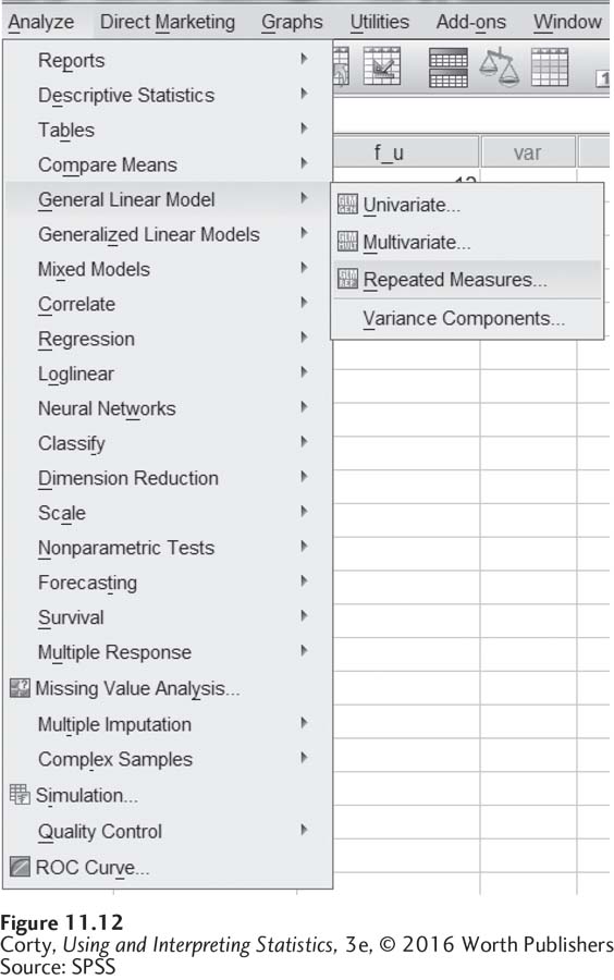
The repeated-measures ANOVA commands are not easy to find in SPSS. They are found under “Analyze” and then “General Linear Model” (see Figure 11.12).
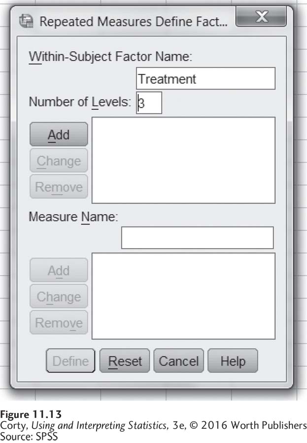
Clicking on “Repeated Measures” opens up a new dialog box, seen in Figure 11.13. “Treatment” is named as the “Within-Subject Factor.” There are three levels of treatment, so the “Number of Levels” is “3.”
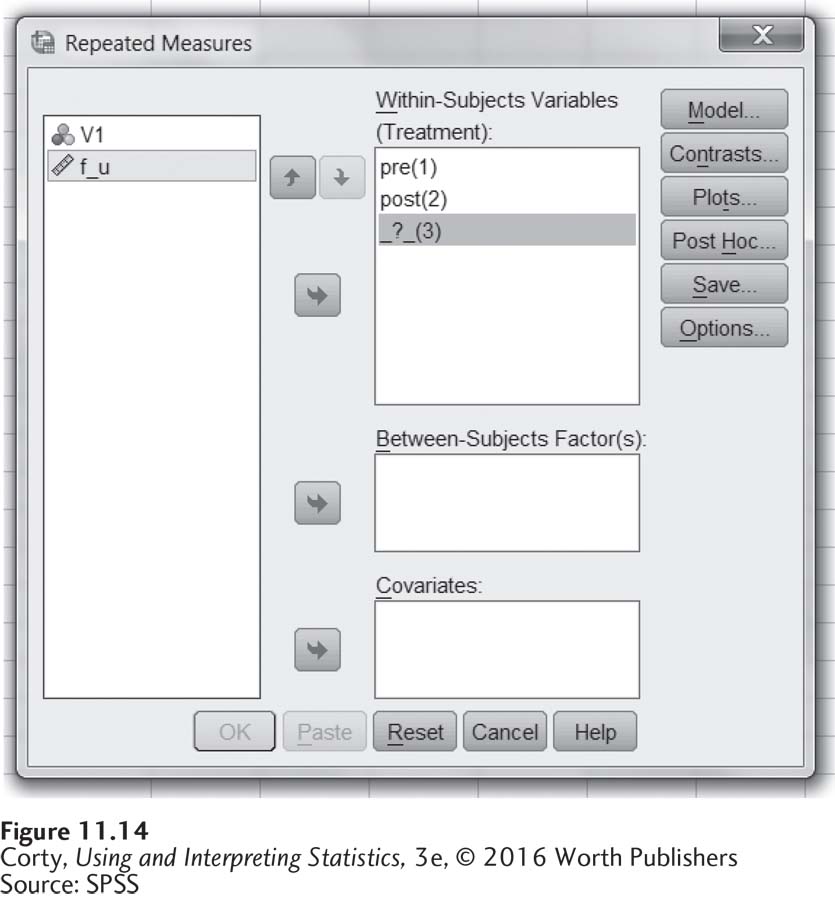
After clicking on the “Add” button (see Figure 11.13), the commands seen in Figure 11.14 open by clicking the “Define” button. Notice that two of the three levels of the “Within-Subjects Variables” are already defined (the variables “pre” and “post”). The third level, “f_u,” is highlighted prior to using the arrow key to send it over.
418
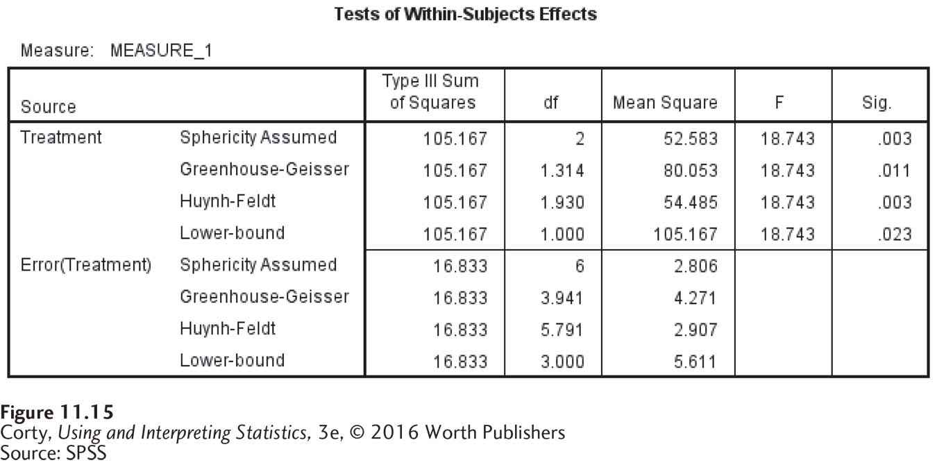
When all three variables have been defined, the “OK” button on the bottom right becomes active. Clicking the OK button causes SPSS to complete the analysis. The printout that SPSS generates for a repeated-measures ANOVA is fairly detailed, but most of the data is not relevant for introductory statistics. Figure 11.15 shows the printout that is most similar to the ANOVA summary table found in Table 11.5.
419
In this summary table, SPSS reports only two sources of variability, the one called treatment and the one called residual. Here, treatment is called “treatment” because it was labeled that way in Figure 11.13. Residual is called “error.” For a basic repeated-measures ANOVA, only pay attention to the first row (of the four rows) for each source, the one labeled “Sphericity Assumed.” The first rows are the only lines with integer values for the degrees of freedom. (The slight differences between values calculated in the text and by SPSS are due to the number of decimal places carried.)
Remember, SPSS reports exact significance levels. Here, the significance level for the F ratio of 18.743 is .003. And .003 ≤ .05, so the results are statistically significant. APA format prefers the use of exact significance levels, so the results would be reported as F (2, 6) = 18.74, p = .003.