12.2 Calculating a Between-Subjects, Two-Way ANOVA
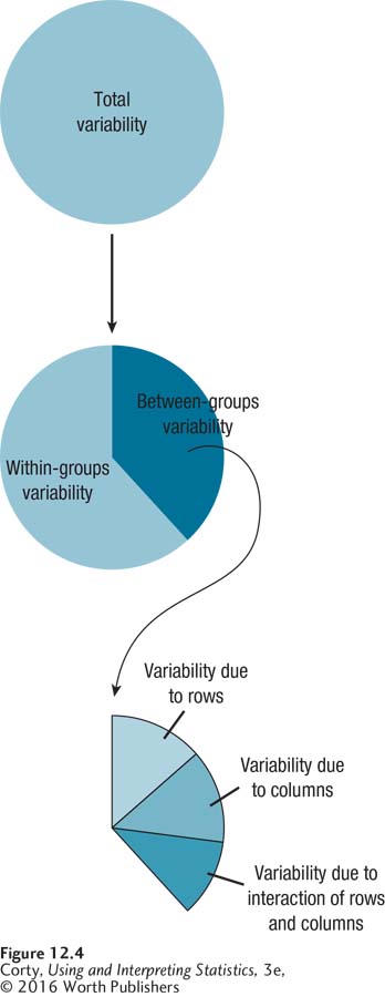
A two-way ANOVA allows a researcher to see, at one time, the effects of two explanatory variables by themselves (the main effects) and in combination (the interaction). A two-way ANOVA achieves this by partitioning the between-group variability differently. As shown in Figure 12.4, a two-way ANOVA takes the total variability and separates that into within-group variability and between-group variability. It then takes the between-group variability and divides that further into the two main effects, the effect of the row explanatory variable and the effect of the column explanatory variable, and the effect of the interaction of the two main effects. Each of these three effects is tested for statistical significance with its own F ratio.
To learn how to complete the calculations for a between-subjects, two-way ANOVA, here’s an example about the effect of caffeine consumption and sleep deprivation on mental alertness. Imagine that a sleep researcher, Dr. Ballard, obtained 30 participants who were students at his college. He gave each a mental alertness task one hour after waking. (Higher scores on this test indicate more mental alertness.) The participants were randomly assigned into six groups, with five in each group. Half the participants consumed a standard cup of coffee (150 mg of caffeine) 30 minutes after waking and half did not. One third of the participants were allowed a full night’s sleep (0-hours sleep deprivation), one third were awakened an hour early (1-hour sleep deprivation), and the final third were awakened two hours early (2-hours sleep deprivation).
431
The design of the study is shown in Table 12.7. Note that the six cells are laid out in a 3 × 2 format as the two explanatory variables are crossed. The two levels for dose of caffeine are the two rows and the three levels for sleep deprivation are the three columns. Each of the 30 participants is in one and only one cell.
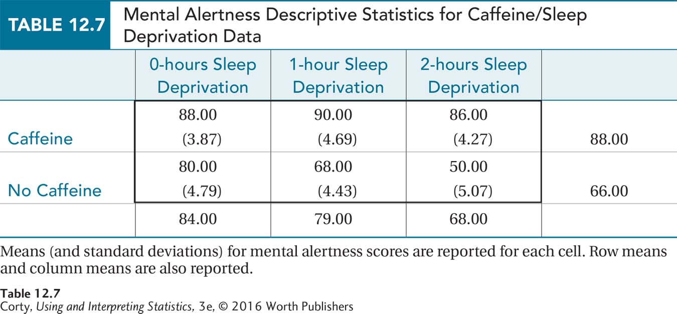
Table 12.7 displays the cell means, row means, and column means, so Dr. Ballard can speculate about main effects. The graph in Figure 12.5 allows him to consider the presence of an interaction.
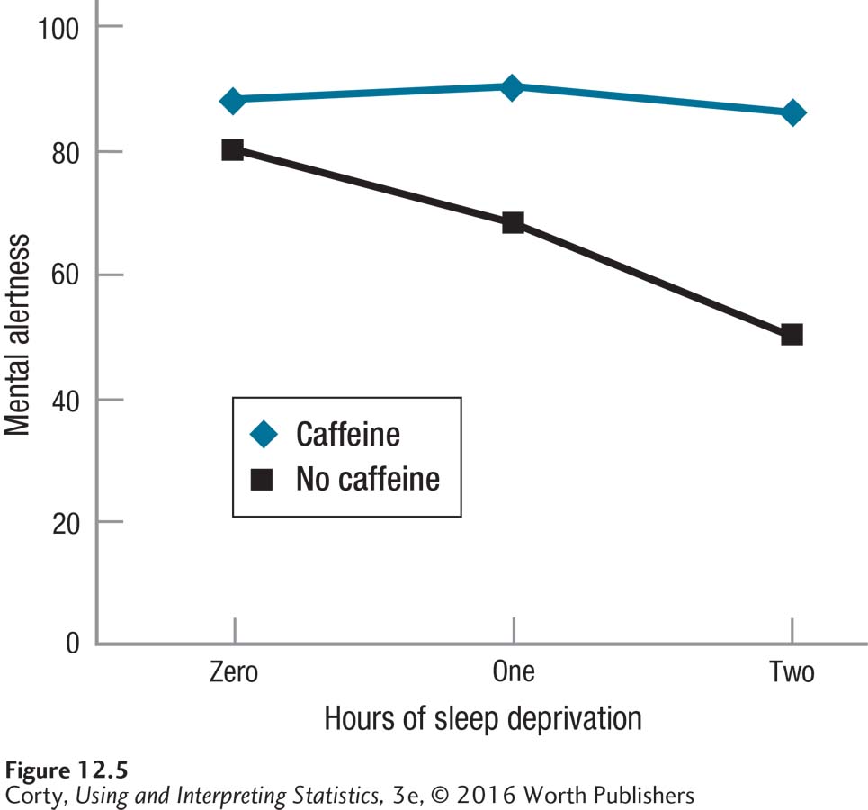
Looking at Table 12.7 and Figure 12.5, three effects are apparent: (1) a main effect for caffeine, with those receiving caffeine performing better; (2) a main effect for sleep deprivation, with those who were more sleep-deprived performing worse; and (3) an interaction between the two variables. Of course, Dr. Ballard will need to do a statistical test to see if any of these results is statistically significant. And, if the interaction effect is statistically significant, that will take precedence over the main effects.
432
Conducting a between-subjects, two-way ANOVA requires following the same six steps for hypothesis testing as in previous hypothesis tests.
Step 1 Pick a Test
Dr. Ballard is comparing the means of six groups, formed by the crossing of two independent variables (caffeine consumption and sleep deprivation). The groups are independent samples, so he’ll use a between-subjects, two-way ANOVA. Specifically, it is a 2 × 3 ANOVA, as there are two levels of caffeine consumption (consume caffeine or not consume caffeine) and three levels of sleep deprivation (0, 1, or 2 hours of deprivation).
433
Step 2 Check the Assumptions

The assumptions for a two-way ANOVA are the same as they are for a between-subjects, one-way ANOVA: random samples, independence of observations, normality, and homogeneity of variance.
Random samples. Dr. Ballard would love to be able to draw a conclusion from his study about humans in general. But, he doesn’t have a random sample of participants from the human population, so the random samples assumption is violated. This is a robust assumption, however, so he can proceed with the two-way ANOVA. He’ll need to be careful about generalizing the results.
Independence of observations. Each participant was tested individually, so their results don’t influence each other and the independence of samples assumption is not violated. This assumption is not robust, so if it had been violated, the analyses couldn’t proceed.
Normality. Dr. Ballard is willing to assume that the dependent variable, mental alertness, is normally distributed in the larger population, so this assumption is not violated. This assumption is robust to violation, especially if the sample size is large.
Homogeneity of variance. All six of the cell standard deviations are about the same (see Table 12.7), which means that the variability in each group is about the same. This assumption is not violated in the study. (And, when the sample size is large, it is a robust assumption.)
For the caffeine/sleep deprivation study, no nonrobust assumptions were violated, so Dr. Ballard can proceed with the ANOVA.
Step 3 List the Hypotheses
For a one-way ANOVA, there is one set of hypotheses. For a two-way ANOVA, with a null hypothesis and an alternative hypothesis for both of the main effects and for the interaction effect, there are three sets of hypotheses.
For the row main effect, the null hypothesis states that the population means for all levels of the row variable are equal to each other. The alternative hypothesis for the row main effect states that not all population means for the levels of the row variable are the same.
For the column main effect, the null hypothesis says that the population means for all levels of the column variable are the same. The alternative hypothesis for the column main effect says that not all population means for the levels of the column variable are the same.
For the interaction effect, the null hypothesis says that there is no interaction effect in the population. This means that the impact of one main effect on the dependent variable is independent of the impact of the other main effect on the dependent variable for all the cells. The alternative hypothesis for the interaction effect says that there is an interaction effect for at least one cell.
434
For the caffeine/sleep deprivation study, the row variable, caffeine consumption, has two levels, so Dr. Ballard writes the hypotheses:
H0 Rows: μRow1 = μRow2
H1 Rows: μRow1 ≠ μRow2
There are three levels of the column variable, sleep deprivation, so the column null hypothesis could be written two ways: (1) μColumn1 = μColumn2 = μColumn3 or (2) all column population means are the same.
H0 Columns: All column population means are the same.
H1 Columns: At least one column population mean is different from
at least one other column population mean.
There is no easy way to write the hypotheses for the interaction effect symbolically. So, using plain language, Dr. Ballard writes the hypotheses as
H0 Interaction: There is no interactive effect of the two independent
variables on the dependent variable in the population.
H1 Interaction: The two independent variables in the population interact
to affect the dependent variable in at least one cell.
Step 4 Set the Decision Rules
Just as three sets of hypotheses exist, there will be three decision rules for a two-way ANOVA—one for the row effect, one for the column effect, and one for the interaction effect. Because this is an ANOVA, F ratios will be calculated for each of the three effects (FRows, FColumns, and FInteraction) and compared to their critical values of F(Fcv Rows, Fcv Columns, and Fcv Interaction). If the observed value of F is greater than or equal to Fcv for an effect, the null hypothesis is rejected for that effect, the alternative hypothesis accepted, and the effect is called statistically significant.
To find a critical value of F for an F ratio, a researcher needs to decide on the alpha level and know the degrees of freedom for the F ratio. The most commonly used alpha levels for ANOVA are .05 and .01, which correspond to a 5% chance and a 1% chance of making a Type I error. (Type I error occurs when the null hypothesis is erroneously rejected.) Typically, alpha is set at .05. When the consequences of a Type I error are more severe, alpha is set at .01 instead. Dr. Ballard, of course, wants to avoid Type I error, but he can live with a 5% chance of it occurring. So, he sets alpha at .05.
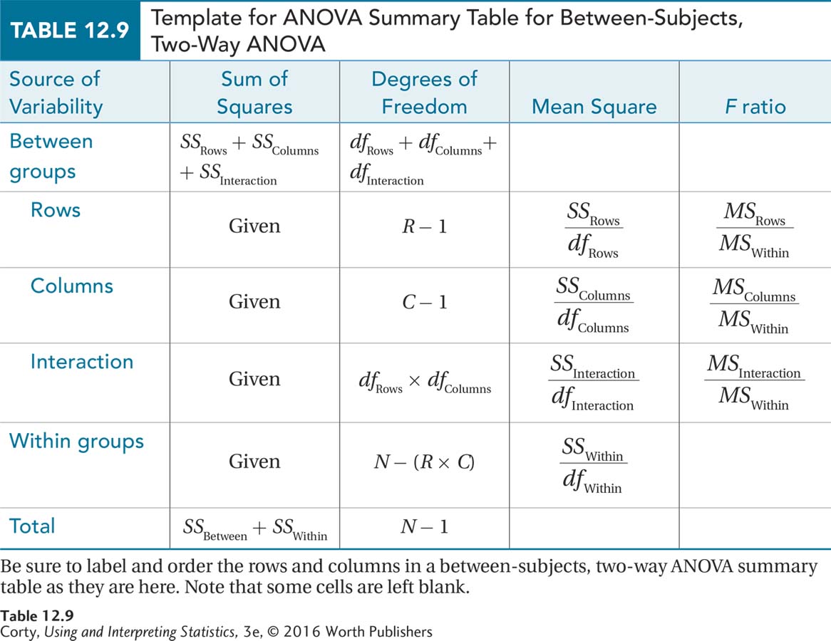
Now he needs to calculate degrees of freedom both for the numerator and the denominator of the F ratios. The degrees of freedom for the numerator will change from F ratio to F ratio, moving from dfRows to dfColumns to dfInteraction as a researcher moves from effect to effect. The degrees of freedom for the denominator term for the between-subjects, two-way ANOVA is degrees of freedom within, dfWithin, and it will remain so across all three of the hypothesis tests. Formulas for calculating all 4 of the degrees of freedom needed to find the critical values of F are shown in Equation 12.2. Table 12.9 (on page 437) shows how to calculate the other 2 degrees of freedom—between groups degrees of freedom and total degrees of freedom—that will be needed to complete the ANOVA summary table.
435
Equation 12.2 Formulas for Calculating Degrees of Freedom for Between-Subjects, Two-Way ANOVA
dfRows = R – 1
dfColumns = C – 1
dfInteraction = dfRows × dfColumns
dfWithin = N – (R × C )
where dfRows = degrees of freedom for the row main effect
dfColumns = degrees of freedom for the column main effect
dfInteraction = degrees of freedom for the interaction effect
dfWithin = degrees of freedom for the within-group effect
R = number of rows
C = number of columns
N = total number of cases
For the caffeine/sleep deprivation study, there are two rows. Here are Dr. Ballard’s calculations for the degrees of freedom for the row main effect:
dfRows = R – 1
= 2 – 1
= 1
With three columns, his calculations for the degrees of freedom for the column main effect look like this:
dfColumns = C – 1
= 3 – 1
= 2
Once dfRows and dfColumns are known, it is easy to calculate the numerator degrees of freedom for the interaction effect:
dfInteraction = dfRows × dfColumns
= 1 × 2
= 2
Finally, checking back and seeing that there were 30 cases, Dr. Ballard calculates the degrees of freedom for the within-group effect:
dfWithin = N – (R × C )
= 30 – (2 × 3)
= 30 – 6
= 24
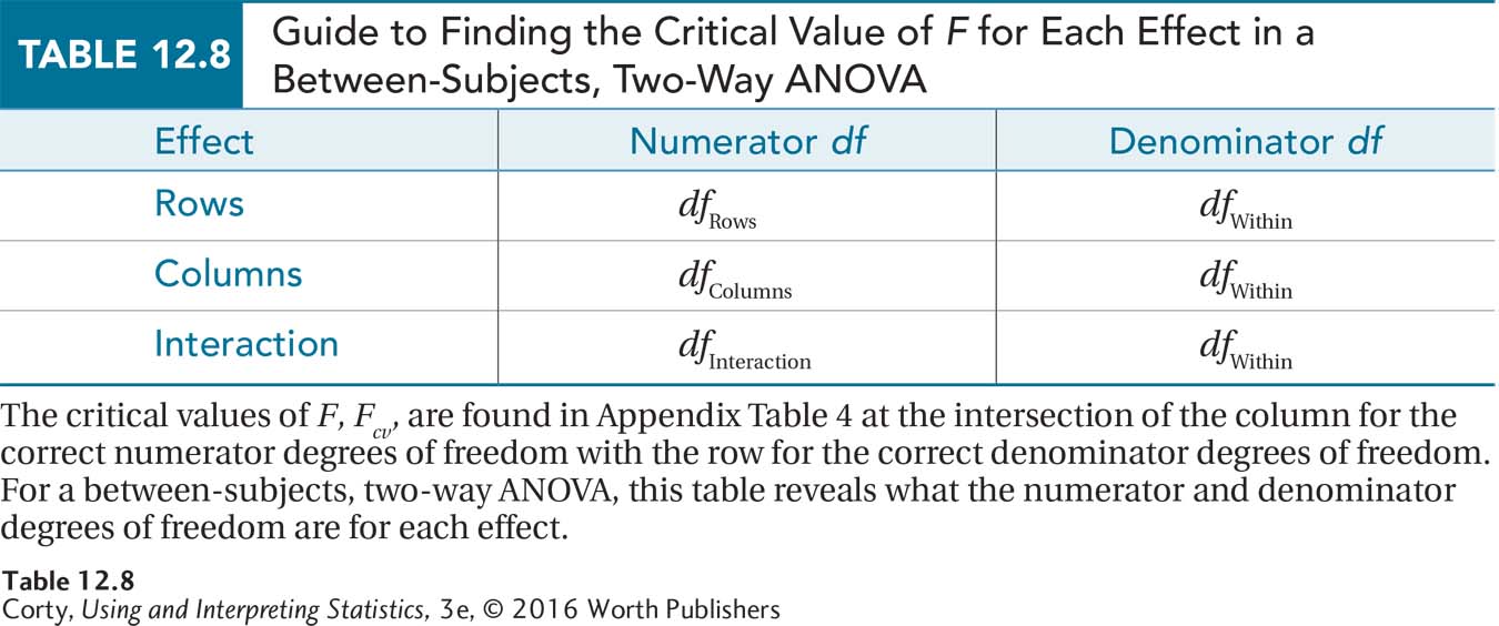
Once all the degrees of freedom have been calculated, they can be used to find the three critical values of F (see Table 12.8). The row main effect has 1 degree of freedom in the numerator, that’s dfRows, and 24 in the denominator, dfWithin. Dr. Ballard looks in Appendix Table 4, at the intersection of the column with 1 degree of freedom and the row with 24 degrees of freedom in the F critical values table for α = .05. There, he finds that the critical value of F, with α = .05, is 4.260 for the row main effect: Fcv Rows = 4.260.
436
Next, he finds the critical value of F for the column main effect. In Appendix Table 4, he uses the column with 2 degrees of freedom and the row with 24 degrees of freedom to find that Fcv for the column effect is 3.403: Fcv Columns = 3.403. The interaction effect has the same numerator and denominator degrees of freedom as the column effect, 2 and 24. So, the critical value of F for the interaction effect is the same as the column effect: Fcv Interaction = 3.403.
Dr. Ballard can now write the decision rules for the three effects for the caffeine/sleep deprivation study as shown:
Row main effect (caffeine)
If FRows ≥ 4.260, reject H0 Rows.
If FRows < 4.260, fail to reject H0 Rows.
Column main effect (sleep deprivation)
If FColumns ≥ 3.403, reject H0 Columns.
If FColumns < 3.403, fail to reject H0 Columns.
Interaction effect
If FInteraction ≥ 3.403, reject H0 Interaction.
If FInteraction < 3.403, fail to reject H0 Interaction.
Step 5 Calculate the Test Statistics
Between-subjects, two-way ANOVA starts the same way between-subjects, one-way ANOVA does. It separates the total variability in a set of scores into between-group variability and within-group variability. Then it goes a step further and separates between-group variability into three subcomponents—variability due to the row effect, variability due to the column effect, and variability due to the interaction effect. Finally, each of these three effects is tested individually with its own F ratio.
The sources of variability in the data are separated out by calculating sums of squares, as was done for the one-way ANOVA. The sums of squares that need to be calculated are:
Sum of squares between groups (SSBetween)
Sum of squares rows (SSRows)
Sum of squares columns (SSColumns)
Sum of squares interaction (SSInteraction)
Sum of squares within groups (SSWithin)
Sum of squares total (SSTotal)
437
Remember that a sum of squares in an ANOVA is a sum of squared deviation scores (see Chapter 11). What scores are used and what mean is subtracted from them vary depending on the source of variability being calculated. The sums of squares are arranged in an ANOVA summary table, Table 12.9, along with the formulas to complete the other necessary values. Note that the same columns that were used for a one-way and repeated-measures ANOVA summary table—source of variability, sum of squares, degrees of freedom, mean square, and F ratio—are present in the same order in the summary table for the two-way ANOVA. But, the sources of variability are different. Making sure that the correct order is followed for the rows and columns in an ANOVA summary table is key to completing an ANOVA. The three effects that are being tested fall under the between-groups effect. Note how they are indented in our table to show that they are derived from the between-groups effect.
Here are the sums of squares for the row effect, the column effect, the interaction effect, and for within-group variability for the caffeine/sleep deprivation study (formulas for calculating sums of squares for a two-way ANOVA are given in an appendix to this chapter):
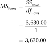
SSRows = 3,630.00
SSBetween = 5,950.00
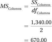
SSColumns = 1,340.00
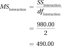
SSInteraction = 980.00
SSWithin = 748.00
SSTotal = 6,698.00
438
Equation 12.2 has already been used to calculate four degrees of freedom—rows, columns, interaction, and within. Table 12.9 shows how to calculate the other two degrees of freedom—between groups and total. Between-groups variability is broken down into variability for rows, columns, and interaction, so degrees of freedom between groups, dfBetween, is found by adding up dfRows, dfColumns, and dfInteraction. For the caffeine/sleep deprivation study, this is
dfBetween = dfRows + dfColumns + dfInteraction
= 1 + 2 + 2
= 5
As shown in Table 12.9, the degrees of freedom total, dfTotal, is calculated by subtracting 1 from the total number of subjects:
dfTotal = N – 1
= 30 – 1
= 29
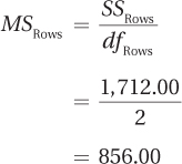
The next step is to calculate mean squares for rows, columns, interaction, and within groups. Following the instructions in Table 12.9:
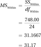
439
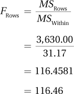
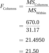
As directed in Table 12.9, Dr. Ballard finds the three F ratios by dividing the mean squares for the row main effect, the column main effect, and the interaction effect by the mean square for within-group variability:
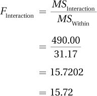
With all the F ratios calculated, the ANOVA summary table is complete (see Table 12.10). We’ll come back to see how the results are interpreted after getting more practice with calculations.
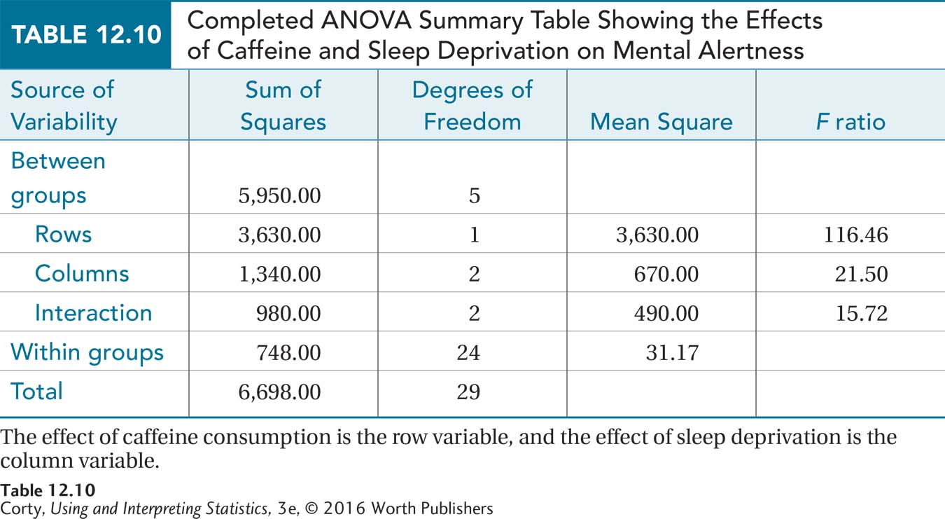
440
Worked Example 12.2
The question “What makes relationships work?” fills the covers of supermarket magazines, but it also interests research psychologists. Dr. Larue, a social psychologist, conducted a study to investigate two variables that she believed were associated with relationship satisfaction. The variables were (1) arguing style and (2) type of parental relationship model.
Dr. Larue found college seniors who were in serious relationships and assessed their ability to argue in a positive or negative way. People who argue positively don’t become threatened or defensive, don’t attack their partners, and help arguments reach a successful conclusion that is satisfactory to both sides. Dr. Larue classified students as positive arguers, mixed arguers, or negative arguers.
Dr. Larue also asked these students to rate the quality of their parents’ marriage as being good, average, or bad. With three levels of parental marital quality and three levels of arguing style, there were nine cells in Dr. Larue’s design. Dr. Larue randomly selected eight students from each cell. That is, there were eight who perceived their parents’ marriages as good and who were positive arguers, eight who rated their parents’ marriages as good and who had a mixed arguing style, and so on. With nine cells and eight participants per cell, Dr. Larue had a total of 72 participants.
Dr. Larue then measured the second grouping variable by asking each student to rate his or her satisfaction with his or her current relationship. (Dr. Larue made sure that no one in the study was in a relationship with someone else in the study.) The interval-level satisfaction scores could range from a low of 5 to a high of 35.
Table 12.11 shows the mean (and standard deviation) for each cell, as well as the row means and the column means. Figure 12.6 displays the data graphically. Looking at Figure 12.6 and Table 12.11 together, there are three things to note:
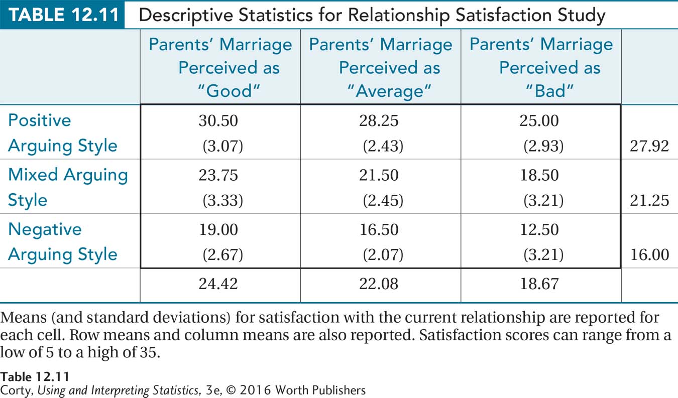
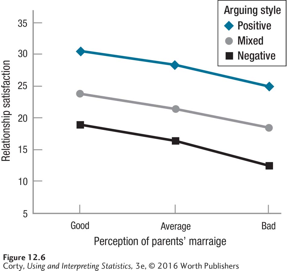
It appears that there is a row main effect for arguing style. Mean satisfaction scores decrease as the amount of negative arguing increases, from 27.92 for positive arguers, to 21.25 for mixed arguers, and 16.00 for negative arguers.
It appears that there is a column main effect for perceived quality of parental marriage. Mean satisfaction scores decrease as the perception of parental marriage becomes more negative, from 24.42 for those with a positive perception, to 22.08 for those with an average perception, and down to 18.67 for those with a negative perception.
441
The three lines are parallel, so there appears to be no interaction between arguing style and quality of parental marriage on relationship satisfaction. Of course, Dr. Larue needs to do a statistical test to see if her observations pan out statistically.
Step 1 Pick a Test. There are two grouping variables (arguing style and parental marriage). Each grouping variable has three levels (positive, mixed, and negative arguing style; good, average, or bad parental marriage). When three levels of arguing style are crossed with three levels of parental marriage, this forms nine groups. Each case is in just one group and each case is not paired with another case, so the groups are all independent. That means this is a between-subjects design. Comparing the means of groups defined by two grouping variables and of groups that are independent samples calls for a between-subjects, two-way ANOVA. Specifically, this is a 3 × 3 ANOVA.
Step 2 Check the Assumptions.
Random samples. The cases used in this study are random samples from the populations of seniors at Dr. Larue’s university who are in relationships and fit in one of the nine cells. This assumption is not violated as long as that is the population to which she wishes to generalize her results.
Independence of observations. No person in the study was in a relationship with anyone else in the study, so this assumption is not violated.
Normality. Dr. Larue is willing to assume that relationship satisfaction is normally distributed within each of the nine populations represented here. Therefore, this assumption is not violated.
Homogeneity of variance. The standard deviations for all nine groups are shown in Table 12.11 and they are all about the same. No standard deviation is twice another, so this assumption is not violated.
Dr. Larue can proceed with the planned statistical test.
442
Step 3 List the Hypotheses. There are three hypotheses in a two-way ANOVA: one for the row main effect (arguing style), one for the column main effect (parental marriage quality), and one for the interaction effect (arguing style × parental marriage quality).
Row main effect:
H0 Rows: μRow1 = μRow2 = μRow3
H1 Rows: At least one row population mean is different
from at least one other.Column main effect:
H0 Columns: μColumn1 = μColumn2 = μColumn3
H1 Columns: At least one column population mean is different
from at least one other.Interaction effect:
H0 Interaction: There is no interactive effect of the two grouping variables
on the dependent variable in the population.H1 Interaction: The two grouping variables interact to affect the
dependent variable in at least one cell in the population.
Step 4 Set the Decision Rules. Setting the decision rules requires deciding on an alpha level and knowing the degrees of freedom for the numerator and the degrees of freedom for the denominator for each of the three effects being tested. Dr. Larue is comfortable having a 5% chance of Type I error, so she sets alpha at .05.
Next, to calculate degrees of freedom, she needs to know R (the number of rows), C (the number of columns), and N (the total number of cases):
R = 3 (There are three levels of arguing style.)
C = 3 (There are three levels of parental marriage quality.)
N = 72 (Each cell has eight cases and there are nine cells: 8 × 9 = 72.)
Using Equation 12.2, Dr. Larue calculates the various degrees of freedom:
dfRows = R – 1
= 3 – 1
= 2
dfColumns = C – 1
= 3 – 1
= 2
dfInteraction = dfRows × dfColumns
= 2 × 2
= 4
dfWithin = N – (R × C)
= 72 – (3 × 3)
= 72 – 9
63
443
Table 12.8 offers guidance as to which source provides the numerator and denominator degrees of freedom for each effect. The critical value of F for the main effect of rows has 2 degrees of freedom in the numerator (dfRows) and 63 degrees of freedom in the denominator (dfWithin). Looking in Appendix Table 4 at the intersection of the column with 2 degrees of freedom and the row with 63 degrees of freedom, Dr. Larue discovers no such row exists. In these situations, apply The Price Is Right rule and use the degrees of freedom value that is closest without going over. Here, that is 60, which makes Fcv Rows = 3.150.
This study has the same degrees of freedom for the numerator and the denominator for the column main effect, 2 and 63. This means Fcv Columns = 3.150.
The degrees of freedom for the numerator for the interaction effect (dfInteraction) are 4 and the denominator degrees of freedom (dfWithin) are 63. Using Table 4 in the Appendix and The Price Is Right rule, Fcv Interaction = 2.525.
Here are Dr. Larue’s three decision rules:
Main effect of rows:
If FRows ≥ 3.150, reject H0 Rows.
If FRows < 3.150, fail to reject H0 Rows.
Main effect of columns:
If FColumns ≥ 3.150, reject H0 Columns.
If FColumns < 3.150, fail to reject H0 Columns.
Interaction effect:
If FInteraction ≥ 2.525, reject H0 Interaction.
If FInteraction < 2.525, fail to reject H0 Interaction.
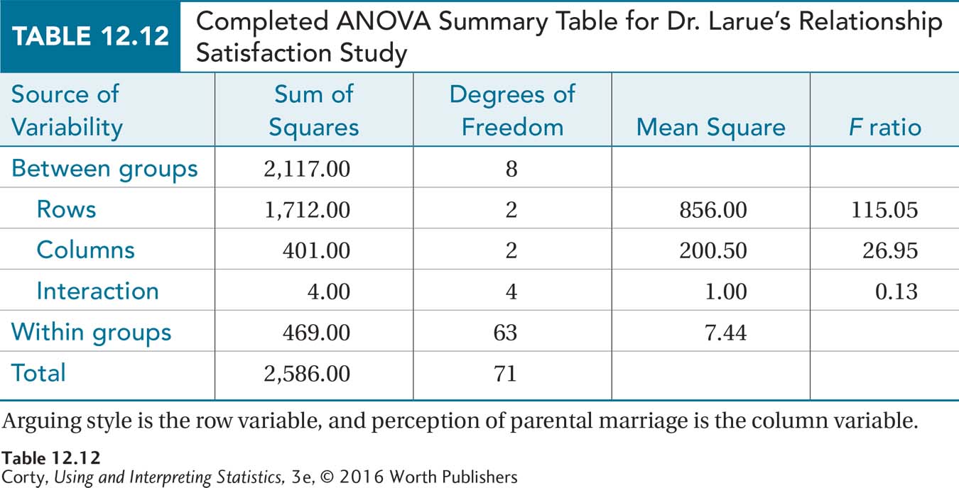
Step 5 Calculate the Test Statistics. Here are the sums of squares for Dr. Larue’s study, derived from the formulas provided in the chapter appendix:
SSBetween = 2,117.00
SSRows = 1,712.00
SSColumns = 401.00
SSInteraction = 4.00
SSWithin = 469.00
SSTotal = 2,586.00
Dr. Larue has already calculated degrees of freedom for rows, columns, interaction, and within groups (2, 2, 4, and 63, respectively), so she can now calculate degrees of freedom for between groups and total degrees of freedom as directed by Table 12.9:
dfBetween = dfRows + dfColumns + dfInteraction
= 2 + 2 + 4
= 8
dfTotal = N – 1
= 72 – 1
= 71
444
The next step is the calculation of the four mean squares. To do this, Dr. Larue divides each of the four sums of squares by its degrees of freedom:
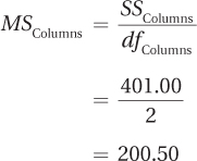
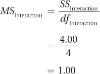
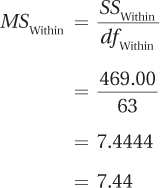
Once the four mean squares have been calculated, all that is left is to find the three F ratios. To do this, Dr. Larue divides each of the mean squares—rows, columns, and interaction—by the mean square within groups:
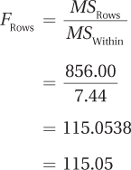
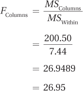
445
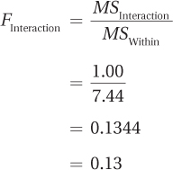
The completed ANOVA summary table is shown in Table 12.12. How to interpret the results found in a summary table is the next order of business.
Practice Problems 12.2
Apply Your Knowledge
12.04 Read each scenario and decide what statistical test should be used. Select from a single-sample z test; single-sample t test; independent-samples t test; paired-samples t test; between-subjects, one-way ANOVA; one-way, repeated-measures ANOVA; and between-subjects, two-way ANOVA.
People who are classified as (1) overweight, (2) normal weight, or (3) underweight are randomly assigned to drink either (1) regular soda, (2) diet soda, or (3) water. Thirty minutes later they indicate, on an interval scale, how thirsty they are.
Backpacks of elementary school students, middle school students, and high school students are weighed to see if there are differences in how heavy they are.
12.05 List the hypotheses for a between-subjects, two-way ANOVA in which there are four rows and three columns.
12.06 Given dfRows = 2, dfColumns = 4, dfInteraction = 8, and dfWithin = 165, list the critical values of F for the three F ratios for a between-subjects, two-way ANOVA for α = .05.
12.07 Given n = 7, R = 2, C = 2, SSBetween = 650.00, SSRows = 250.00, SSColumns = 300.00, SSInteraction = 100.00, SSWithin = 800.00, and SSTotal = 1,450.00, complete an ANOVA summary table for a between-subjects, two-way ANOVA.