CHAPTER EXERCISES
Answers to the odd-numbered exercises appear in Appendix B.
Review Your Knowledge
12.01 ____-way ANOVA examines the impact of two explanatory variables at the same time.
12.02 A 2 × 3 ANOVA could also be called a ____ × ____ ANOVA.
12.03 “Between subjects” means ____ samples and “____ subjects” means dependent samples.
12.04 Two-way ANOVA, three-way ANOVA, and four-way ANOVA are all examples of ____ ANOVA.
12.05 There is an advantage in performing one ____-way ANOVA over two ____-way ANOVAs.
12.06 If every level of one explanatory variable occurs with every level of the other explanatory variable, then the two explanatory variables are said to be ____.
12.07 A two-way ANOVA has two ____ effects and one ____ effect.
12.08 An interaction occurs when the effect of one explanatory variable on the dependent variable ____ on the level of the other explanatory variable.
12.09 If the lines in a graph are ____, then an interaction exists.
12.10 If each cell has the same sample size, the cell means in a row can be averaged to find the ____.
12.11 Row means and column means give information about ____ effects.
12.12 If the interaction effect is statistically significant, ____ interpret the main effects.
12.13 In a between-subjects, two-way ANOVA, the groups are ____ samples.
12.14 The random samples assumption says that the sample is a ____ from the ____ to which one wishes to generalize the results.
12.15 If cases in a cell influence each other’s scores on the dependent variable, then the ____ assumption is violated.
12.16 The ____ assumption is tested by looking at cell standard deviations.
12.17 In a two-way ANOVA, there are ____ sets of hypotheses.
12.18 The row’s null hypothesis states that the ____ for all levels of the row variable are equal.
12.19 The alternative hypothesis for the columns says that ____ one of the population column means differs from ____ one of the other population column means.
12.20 The alternative hypothesis for the interaction effect says that there is ____ for at least one cell.
12.21 Decision rules exist for the columns main effect, the rows main effect, and the ____.
464
12.22 The decision rule for the interaction effect involves comparing FInteraction to ____.
12.23 The number of degrees of freedom for the row effect depends on ____.
12.24 The denominator degrees of freedom for all the F ratios calculated for a between-subjects, two-way ANOVA is degrees of freedom ____.
12.25 Finding Fcv in Appendix Table 4 depends on knowing the numerator ____ and denominator ____ for the F ratio.
12.26 If FInteraction < Fcv Interaction, then the null hypothesis is ____.
12.27 Total variance in between-subjects, two-way ANOVA is divided into two factors: ____ and ____.
12.28 In between-subjects, two-way ANOVA, between-group variability is divided into variability due to ____, ____, and ____.
12.29 SS is the abbreviation for a sum of ____.
12.30 To calculate a mean square, one divides a ____ by its ____.
12.31 MSInteraction divided by MSWithin calculates ____.
12.32 When an ANOVA summary table for a between-subjects, two-way ANOVA is completed, there are ____ F ratios.
12.33 If a null hypothesis is rejected, the result is called ____.
12.34 If results, in APA format, are written as p > .05, the null hypothesis was ____.
12.35 p < .05 means that alpha was set at ____.
12.36 Only interpret a main effect if ____.
12.37 ____ is the effect size used for between-subjects, two-way ANOVA.
12.38 Eta squared is calculated for both ____ effects and for the ____.
12.39 An effect of ≈ ____% is considered a medium effect.
12.40 Eta squared can alert one to the risk of ____ error if the effect was not statistically significant.
12.41 Post-hoc tests should only be used when an effect is ____.
12.42 If the row main effect is statistically significant and there are only two rows, it is/is not necessary to do a post-hoc test for the row effect.
12.43 If two cells differ by exactly the HSD amount, then the difference is ____.
12.44 The HSD value for the interaction effect is used to compare ____ means.
Apply Your Knowledge
Select the right test for the scenario from among a single-sample z test; single-sample t test; independent-samples t test; paired-samples t test; between-subjects, one-way ANOVA; one-way, repeated-measures ANOVA; and between-subjects, two-way ANOVA.
12.45 A dentist randomly assigns people to use one of three different forms of dental hygiene: (1) dental floss, (2) wooden toothpicks, or (3) anti-plaque rinse. After six months he measures, in grams, how much plaque he scrapes off the teeth. What statistical test should he use to see if form of dental hygiene has an impact on the amount of plaque?
12.46 The American Psychological Association wanted to determine if there was a difference in post-graduation success between BA and BS degrees in psychology. It put together a random sample of students with each degree and found out what the annual salary was for their first job after graduation. What statistical test should be used to analyze these data for the effect of type of degree?
12.47 Male and female athletes exercised for an hour on a treadmill. During this time, half of each sex was assigned to drink water and half was assigned to drink a sport beverage. At the end of the hour, lactic acid levels were measured and mean levels were calculated. What statistical test should be used to see how sex and type of beverage affect lactic acid production?
465
12.48 To study accommodation to the loss of an eye, a sensory psychologist obtained 10 volunteers who agreed to wear an eye patch over one eye for 4 weeks. To test visual ability, the psychologist used a batting test: a pitching machine lobbed 50 pitches to each participant and the psychologist counted how many were hit. This test was conducted (a) before the eye patch was worn, (b) immediately after the eye patch was first put on, (c) 1 week into the study, (d) 2 weeks into the study, (e) 3 weeks into the study, (f) on the last day wearing the eye patch, and (g) 1 week later. What test should be used to see if batting ability changed over the course of the study?
Calculating row and column means
12.49 There are 10 participants in each cell. Each cell is an independent sample. The design is fully crossed. The value in each cell is the cell mean. Calculate (a) row means and (b) column means for this matrix.
| Column 1 | Column 2 | Column 3 | |
| Row 1 | 25 | 35 | 45 |
| Row 2 | 25 | 15 | 5 |
12.50 There are 17 participants in each cell. Each cell is an independent sample. The design is fully crossed. The value in each cell is the cell mean. Calculate (a) row means and (b) column means for this matrix.
| Column 1 | Column 2 | Column 3 | |
| Row 1 | 100 | 110 | 140 |
| Row 2 | 140 | 200 | 180 |
Speculating about main effects and interactions
12.51 Given the cell means, row means, and column means below, (a) graph the results to examine if there is an interaction; (b) speculate about which effects would be statistically significant; (c) indicate which effects should be interpreted.
| Column 1 | Column 2 | ||
| Row 1 | 17 | 13 | 15.00 |
| Row 2 | 16 | 12 | 14.00 |
| 16.50 | 12.50 |
12.52 Given the cell means, row means, and column means below, (a) graph the results to determine if you think there is an interaction; (b) speculate about which effects would be statistically significant; (c) indicate which effects should be interpreted.
| Column 1 | Column 2 | ||
| Row 1 | 80 | 60 | 70.00 |
| Row 2 | 60 | 40 | 50.00 |
| 70.00 | 50.00 |
Checking the assumptions
12.53 Eighty volunteers who read about a study in a newspaper were randomly assigned to be in the experimental or control group. Within each group, participants were randomly assigned to one of four different conditions. Each participant then participated in the study individually. After this, each participant’s status on the interval-level psychological variable was measured. Below are the means (and standard deviations). (a) Evaluate all four assumptions and (b) decide if it is OK to proceed with the test.
| I | II | III | IV | |
| Control | 12.34 (2.89) | 13.76 (3.89) | 14.17 (4.95) | 16.88 (6.91) |
| Experimental | 14.88 (3.12) | 15.66 (4.18) | 16.99 (5.54) | 17.33 (6.48) |
12.54 A researcher was interested in the impact of different types of day care on children’s development. She obtained samples of children who (a) had been watched by a babysitter at home; (b) had attended small, home-based day care; or (c) had gone to a large day-care center. She also classified the children as having received paid care for (1) less than 40 hours a week or (2) 40 or more hours per week. There were eight children in each cell and no siblings were included. She measured each child’s adjustment level, on an interval scale, in the first grade. Below are the means (and standard deviations). (a) Evaluate all four assumptions and (b) decide if it is OK to proceed with the test.
466
| Babysitter | Small Day Care | Large Day Care | |
| <40 Hours | 112.66 (14.83) | 108.28 (16.76) | 106.80 (17.65) |
| ≥40 Hours | 114.88 (13.12) | 108.71 (15.66) | 109.28 (16.77) |
Listing hypotheses
12.55 List all the hypotheses for the ANOVA described in Exercise 12.53 for (a) rows, (b) columns, and (c) interaction.
12.56 List all the hypotheses for the ANOVA described in Exercise 12.54 for (a) rows, (b) columns, and (c) interaction.
Calculating degrees of freedom
12.57 If R = 3, C = 4, and n = 8, calculate the degrees of freedom for the following effects: (a) rows, (b) columns, (c) interaction, (d) within groups, (e) between groups, and (f) total.
12.58 If R = 2, C = 3, and n = 11, calculate the degrees of freedom for the following effects: (a) rows, (b) columns, (c) interaction, (d) within groups, (e) between groups, and (f) total.
Finding Fcv
12.59 If α = .05, dfRows = 2, dfColumns = 2, dfInteraction = 4, and dfWithin = 36, find (a) Fcv Rows, (b) Fcv Columns, and (c) Fcv Interaction.
12.60 If α = .05, dfRows = 3, dfColumns = 1, dfInteraction = 3, and dfWithin = 40, find (a) Fcv Rows, (b) Fcv Columns, and (c) Fcv Interaction.
Writing the decision rule
12.61 If Fcv Interaction is 2.668, what is the decision rule for the interaction effect?
12.62 If Fcv Rows is 3.295, what is the decision rule for the rows effect?
Calculating mean squares
12.63 If SSWithin = 168.48 and dfWithin = 40, calculate MSWithin.
12.64 If SSInteraction = 0.60 and dfInteraction = 4, calculate MSInteraction.
Calculating F ratios
12.65 If MSRows = 17.30 and MSWithin = 3.33, what is FRows?
12.66 If MSColumns = 66.54 and MSWithin = 78.88, what is FColumns?
Completing a summary table
12.67 Given R = 2, C = 2, n = 5, SSBetween = 61.00, SSRows = 15.00, SSColumns = 12.00, SSInteraction = 34.00, SSWithin = 120.00, and SSTotal = 181.00, complete the ANOVA summary table for a between-subjects, two-way ANOVA.
12.68 Given R = 2, C = 4, n = 12, SSBetween = 225.00, SSRows = 78.00, SSColumns = 23.00, SSInteraction = 124.00, SSWithin = 350.00, and SSTotal = 575.00, complete the ANOVA summary table for a between-subjects, two-way ANOVA.
Applying the decision rule
12.69 If Fcv = 3.443 and F = 17.55, was the null hypothesis rejected?
12.70 If Fcv = 3.191 and F = 2.86, was the null hypothesis rejected?
Writing results in APA format
12.71 If FInteraction = 3.70, dfInteraction = 2, dfWithin = 66, and Fcv Interaction = 3.138, write the results in APA format. Use α = .05.
12.72 If FRows = 2.87, dfRows = 2, dfWithin = 171, and Fcv Rows = 3.053, write the results in APA format. Use α = .05.
12.73 If FColumns = 2.45, dfColumns = 3, and dfWithin = 168, write the results in APA format. Use α = .05.
12.74 If FColumns = 4.00, dfColumns = 1, and dfWithin = 36, write the results in APA format. Use α = .05.
12.75 Given the ANOVA summary table below, write the results in APA format for (a) the rows effect, (b) the columns effect, and (c) the interaction effect. Use α = .05.
467
| Source of Variability | Sum of Squares | Degrees of Freedom | Mean Square | F ratio |
| Between groups | 108.56 | 5 | ||
| Rows | 45.40 | 2 | 22.70 | 3.21 |
| Columns | 7.62 | 1 | 7.62 | 1.08 |
| Interaction | 55.54 | 2 | 27.77 | 3.93 |
| Within groups | 212.22 | 30 | 7.07 | |
| Total | 320.78 | 35 |
12.76 Given the ANOVA summary table below, write the results in APA format for (a) the rows effect, (b) the columns effect, and (c) the interaction effect. Use α = .05.
| Source of Variability | Sum of Squares | Degrees of Freedom | Mean Square | F ratio |
| Between groups | 70.40 | 7 | ||
| Rows | 32.34 | 3 | 10.78 | 2.77 |
| Columns | 7.62 | 1 | 7.62 | 1.96 |
| Interaction | 30.44 | 3 | 10.15 | 2.61 |
| Within groups | 342.66 | 88 | 3.89 | |
| Total | 413.06 | 95 |
Deciding which effects to interpret
12.77 If the null hypothesis is rejected for all three effects (rows, columns, and interaction), which effects should be interpreted?
12.78 If the null hypothesis is rejected for the rows effect and the columns effect but not for the interaction effect, which effects should be interpreted?
12.79 If the null hypothesis is rejected for the interaction effect but not for the rows effect or the columns effect which effects should be interpreted?
12.80 If the null hypothesis is rejected for the rows effect and the interaction effect but not for the columns effect, which effects should be interpreted?
Calculating eta squared
12.81 If SSRows = 3.78 and SSTotal = 47.83, (a) calculate η2Rows and (b) classify the effect as small, medium, or large.
12.82 If SSColumns = 17.91 and SSTotal = 783.54, (a) calculate η2Columns and (b) classify the effect as small, medium, or large.
12.83 Given the ANOVA summary table below, calculate η2 for (a) the rows effect, (b) the columns effect, and (c) the interaction effect.
| Source of Variability | Sum of Squares | Degrees of Freedom | Mean Square | F ratio |
| Between groups | 132.00 | 7 | ||
| Rows | 33.00 | 3 | 11.00 | 4.56 |
| Columns | 54.00 | 1 | 54.00 | 22.41 |
| Interaction | 45.00 | 3 | 15.00 | 6.22 |
| Within groups | 212.00 | 88 | 2.41 | |
| Total | 344.00 | 95 |
12.84 Given the ANOVA summary table below, calculate η2 for (a) the rows effect, (b) the columns effect, and (c) the interaction effect.
| Source of Variability | Sum of Squares | Degrees of Freedom | Mean Square | F ratio |
| Between groups | 125.00 | 5 | ||
| Rows | 45.00 | 2 | 22.50 | 18.29 |
| Columns | 68.00 | 1 | 68.00 | 55.28 |
| Interaction | 12.00 | 2 | 6.00 | 4.88 |
| Within groups | 140.00 | 114 | 1.23 | |
| Total | 265.00 | 119 |
Finding q
12.85 Given R = 3, C = 2, and n = 8, find (a) qRows, (b) qColumns, and (c) qCells.
12.86 Given R = 3, C = 3, and n = 11, find (a) qRows, (b) qColumns, and (c) qCells.
Calculating HSD
12.87 If qRows = 3.49, MSWithin = 4.56, and nRows = 12, what is HSDRows?
12.88 If qCells = 2.96, MSWithin = 12.75, and nCells = 4, what is HSDCells?
468
12.89 If α = .05, for which effects should an HSD value be calculated?
| Source of Variability | Sum of Squares | Degrees of Freedom | Mean Square | F ratio |
| Between groups | 324.00 | 8 | ||
| Rows | 70.00 | 2 | 35.00 | 28.46 |
| Columns | 88.00 | 2 | 44.00 | 35.77 |
| Interaction | 166.00 | 4 | 41.50 | 33.74 |
| Within groups | 100.00 | 81 | 1.23 | |
| Total | 424.00 | 89 |
12.90 If α = .05, for which effects should an HSD value be calculated?
| Source of Variability | Sum of Squares | Degrees of Freedom | Mean Square | F ratio |
| Between groups | 118.00 | 8 | ||
| Rows | 88.00 | 2 | 44.00 | 9.91 |
| Columns | 23.00 | 2 | 11.50 | 2.59 |
| Interaction | 7.00 | 4 | 1.75 | 0.39 |
| Within groups | 600.00 | 135 | 4.44 | |
| Total | 718.00 | 143 |
Interpreting HSD
12.91 If MRow 1 = 117.66, MRow 2 = 113.63, MRow 3 = 128.91, and HSDRows = 5.89, determine (a) which rows have a statistically significant difference and (b) the direction of the differences.
12.92 If MCell 1 = 55.54, MCell 2 = 48.34, MCell 3 = 36.44, MCell 4 = 59.40, and HSDCells = 7.83, determine (a) which cells have a statistically significant difference and (b) the direction of the differences.
Interpreting results
12.93 A consumer psychologist classified shoppers at a grocery store as (a) being males or females, and (b) shopping with or without children. These two variables were crossed and he took a random sample of five shoppers from each of the four cells. Then he gave them the Enjoyment of Shopping Experience Scale (ESES) to be completed for the current shopping experience. The ESES is an interval-level measure, with a mean of 50 indicating neutral feelings about shopping. Scores can range from 20 to 80, with scores above 50 an indication of enjoying shopping; scores below 50 indicate that shopping is not enjoyable. Here are the means:
| Shopping Without Children | Shopping With Children | Row Means | |
| Male Shopper | 43.20 | 56.80 | 50.00 |
| Female Shopper | 57.40 | 44.80 | 51.10 |
| Column Means | 50.30 | 50.80 |
No nonrobust assumptions were violated and a between-subjects, two-way ANOVA was completed. Here is the ANOVA summary table:
| Source of Variability | Sum of Squares | Degrees of Freedom | Mean Square | F ratio |
| Between groups | 865.35 | 3 | ||
| Rows | 6.05 | 1 | 6.05 | 0.29 |
| Columns | 1.25 | 1 | 1.25 | 0.06 |
| Interaction | 858.05 | 1 | 858.05 | 41.15 |
| Within groups | 333.60 | 16 | 20.85 | |
| Total | 1,198.95 | 19 |
The researcher calculated η2Rows = 0.50%, η2Columns = 0.10%, η2Interaction = 71.57%, and HSDCells = 8.27. Complete a four-point interpretation for the results. (Hint: Graphing the results will help.)
12.94 A cognitive psychologist decided to investigate whether two beliefs about healthy living had any real impact on performance in college. She took 40, first-semester college student volunteers and randomly assigned half to eat breakfast every day and the other half to skip breakfast every day. This was crossed with another variable. Half the students were randomly assigned to sleep at least 8 hours a night and half were randomly assigned to sleep less than 8 hours a night. At the end of the semester, she recorded each participant’s GPA. The results are shown in this table:
469
| Sleep ≥8 Hours | Sleep <8 Hours | Row Means | |
| Eat Breakfast | 3.20 | 2.72 | 2.96 |
| Skip Breakfast | 3.08 | 2.77 | 2.93 |
| Column Means | 3.14 | 2.75 |
No nonrobust assumptions for a between-subjects, two-way ANOVA were violated and the ANOVA was completed. Here is the summary table:
| Source of Variability | Sum of Squares | Degrees of Freedom | Mean Square | F ratio |
| Between groups | 1.64 | 3 | ||
| Rows | 0.01 | 1 | 0.01 | 0.06 |
| Columns | 1.56 | 1 | 1.56 | 9.18 |
| Interaction | 0.07 | 1 | 0.07 | 0.41 |
| Within groups | 6.03 | 36 | 0.17 | |
| Total | 7.67 | 39 |
The eta squared values for rows, columns, and interaction are, respectively, 0.13%, 20.34%, and 0.91%. HSDCells is 0.50. Interpret the results. (Hint: Graphing the results will help.)
12.95 A developmental psychologist investigated the influence of two crossed variables—exposure to televised violence and type of parental discipline—on teens’ acceptance of violence. He obtained a random sample of seniors at the local high school and classified them on two dimensions: (1) whether or not their parents had restricted their television viewing and (2) whether their parents used positive reinforcement or punishment. He took a random sample of six teens from each of the four samples (no siblings were included) and his dependent variable was each teen’s score on the interval-level Approval of Violence Scale (AVS). Scores on the AVS range from 0 to 20, with higher scores indicating a greater acceptance of violence as a way to solve disagreements. The cell means (and standard deviations) are shown below. SSRows was calculated to be 210.04, SSColumns as 222.04, SSInteraction as 15.04, and SSWithin as 204.83.
| Restricted TV | Unrestricted TV | |
| Positive Reinforcement | 6.00 (2.10) | 10.50 (3.62) |
| Punishment | 10.33 (4.08) | 18.00 (2.61) |
12.96 An industrial organizational psychologist investigated the crossed effects of two variables—being a member of a team sport in high school and extroversion level—on how well professors are liked by their colleagues. The dependent variable was the interval-level Colleague Collegiality Scale (CCS). Scores on the CCS range from 0 to 24; higher scores indicate greater liking by colleagues. From a national and representative sample of college professors, the psychologist randomly selected professors until there were eight in each cell. The table below shows the cell means (and standard deviations). SSRows was 36.13, SSColumns = 1.13, SSInteraction = 36.13, and SSWithin = 217.50.
| Extroverted | Introverted | |
| Played a Team Sport in High School | 16.50 (2.51) | 14.00 (2.39) |
| Did Not Play a Team Sport in High School | 12.25 (3.62) | 14.00 (2.45) |
Expand Your Knowledge
12.97 Each cell in the table contains seven cases. (a) Given the cell, row, and column means below, calculate the missing cell means. If it can’t be done, say so. (b) Calculate the mean for all 28 cases. If it can’t be done, say so.
| Condition 1 | Condition 2 | Row Means | |
| Control Group | A 4.00 | B | 8.00 |
| Experimental Group | C | D | 7.00 |
| Column Means | 6.00 | 9.00 |
470
12.98 Each cell in this table has the same number of cases, but that number is unknown. (a) Given the cell, row, and column means below, calculate the missing cell means. If it can’t be done, say so. (b) Calculate the mean for all the cases. If it can’t be done, say so.
| Condition 1 | Condition 2 | Row Means | |
| Control Group | A | B | 6.00 |
| Experimental Group | C 5.00 | D | 5.50 |
| Column Means | 7.00 | 4.50 |
12.99 Each cell in the table has five cases. (a) Given the cell, row, and column means below, calculate the missing cell means. If it can’t be done, say so. (b) Calculate the mean for all 30 cases. If it can’t be done, say so.
| Condition 1 | Condition 2 | Condition 3 | Row Means | |
| Control Group | A 1.00 | B | C | 2.00 |
| Experimental Group | D | E | F | 6.00 |
| Column Means | 2.50 | 5.50 | 4.00 |
12.100 The means of five independent samples are being compared. Which ANOVA is being used?
between-subjects, one-way ANOVA
one-way, repeated-measures ANOVA
between-subjects, two-way ANOVA
(a) or (b)
(a) or (c)
not enough information provided to decide
12.101 The means of six independent samples are being compared. Which ANOVA is being used?
between-subjects, one-way ANOVA
one-way, repeated-measures ANOVA
between-subjects, two-way ANOVA
(a) or (b)
(a) or (c)
not enough information provided to decide
12.102 Given R = 3, C = 3, n = 12, and the ANOVA summary table below, calculate HSD values for the effects as necessary and appropriate.
| Source of Variability | Sum of Squares | Degrees of Freedom | Mean Square | F ratio |
| Between groups | 184.00 | 8 | ||
| Rows | 115.00 | 2 | 57.50 | 9.49 |
| Columns | 12.00 | 2 | 6.00 | 0.99 |
| Interaction | 57.00 | 4 | 14.25 | 2.35 |
| Within groups | 600.00 | 99 | 6.06 | |
| Total | 784.00 | 107 |
12.103 If SSRows = 17.50, SSColumns = 13.75, SSInteraction = 22.25, and SSWithin = 44.75, calculate (a) SSBetween and (b) SSTotal.
12.104 If SSRows = 123.60, SSColumns = 80.30, SSInteraction = 20.80, and SSWithin = 168.20, calculate (a) SSBetween and (b) SSTotal.
SPSS
Data to be analyzed for a between-subjects, two-way ANOVA with SPSS have to be entered in the data editor in a certain manner. Each case goes on a separate row and each of the three variables—the two independent variables and the one dependent variable—has a column. Figure 12.11 shows how the caffeine/sleep deprivation data are entered.
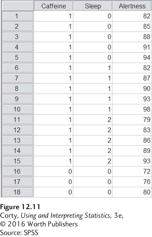 Figure 12.31: Figure 12.11 Data Entry for Between-Subjects, One-Way ANOVA for SPSS Each case is on a separate row. The values for the two independent variables and for the dependent variable fall in the columns.(Source: SPSS)
The first column contains the data for the independent variable “Caffeine,” which has two levels. Cases who consumed caffeine have a value of 1 and those who did not consume caffeine are given a value of 0.
471
The second column, “Sleep,” contains information about which amount of sleep deprivation a case has experienced. Those with no sleep deprivation have the value of 0, one hour of sleep deprivation gets a 1, and two hours of sleep deprivation gets a 2.
The third column, “Alertness,” is the case’s score on the mental alertness task.
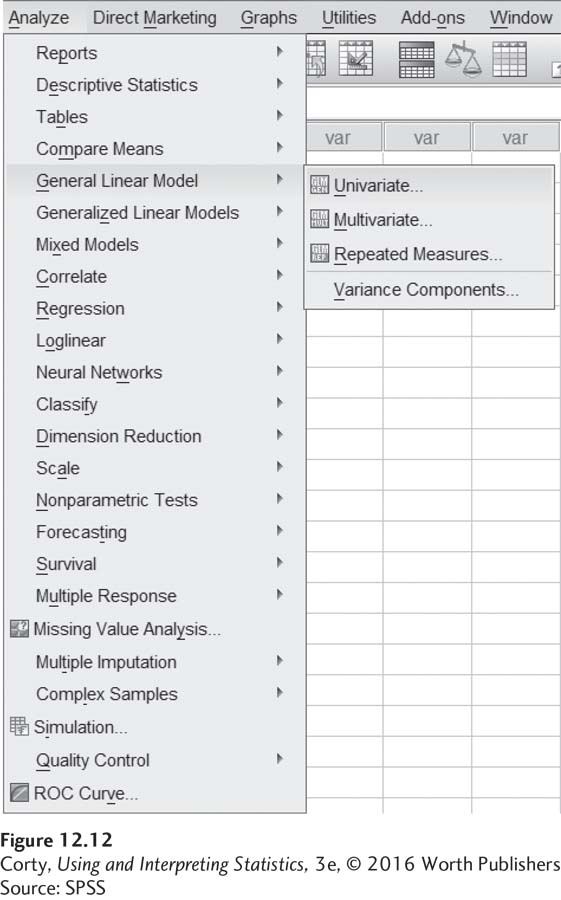
There are two menus that must be accessed to run a between-subjects, two-way ANOVA in SPSS. To start, as shown in Figure 12.12, click on “Analyze,” then “General Linear Model,” and then “Univariate. . . .”
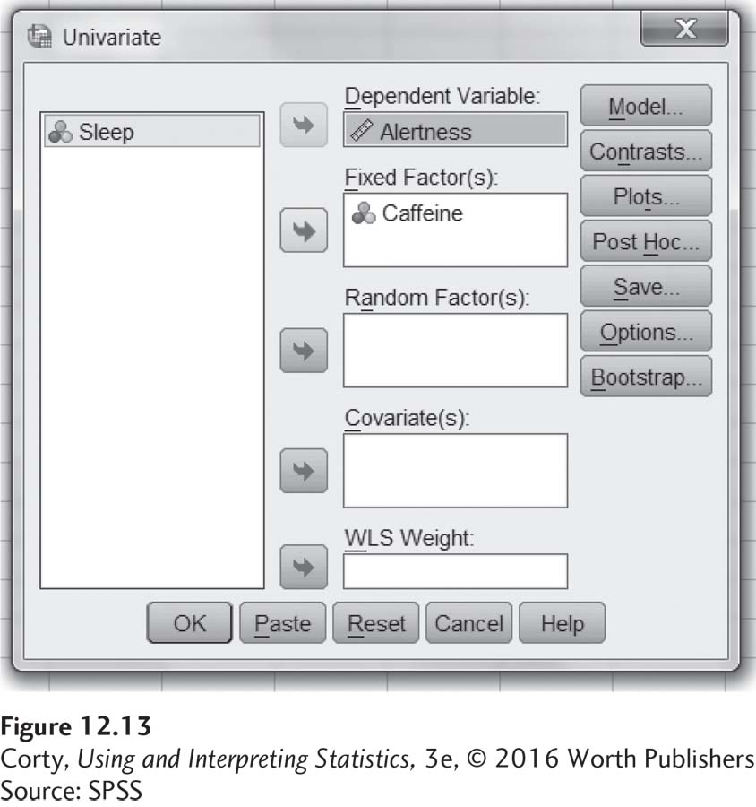
Clicking on “Univariate. . .” opens up the menu seen in Figure 12.13. Note that the arrow buttons have already been used to send “Alertness” to the dependent variable box and “Caffeine” to the fixed factors box. Once the arrow button is used to send “Sleep” to the fixed factors box, press the “Go” button at the bottom to initiate the calculations.
472
The results are seen in Figure 12.14. The SPSS ANOVA summary table is arranged a little differently from the one in the text. The columns in the summary table are the same, but there is one additional column labeled “Sig.” This gives the exact significance level for an F ratio.
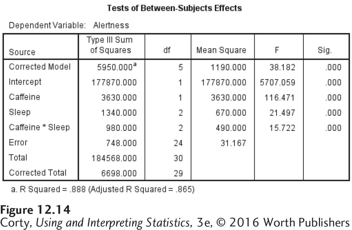
The rows in the summary table have some different sources of variability. Focus on the three that are labeled “Caffeine,” “Sleep,” and “Caffeine * Sleep.”
The row labeled “Caffeine” gives the results for the main effect of the caffeine variable.
The row labeled “Sleep” gives the results for the main effect of the sleep deprivation variable.
473
The interaction effect is the one in which the two main effects are connected with an asterisk, “Caffeine * Sleep.”
The row labeled “Error” is what the text calls “Within.” This is the denominator term for all three of the F ratios.
The F ratios calculated by SPSS have one more decimal place than those calculated in this book, but otherwise they are the same. The final column in the summary table gives the exact significance level for an effect. If the alpha level is set at .05, then a result is statistically significant as long as the significance level reported in this column is ≤.05.