14.2 Errors in Regression
The goal of regression is to be able to predict Y values for X values. And the more accurately this can be done, the better. That’s why researchers need a way to measure how much error occurs in prediction. As we’ll soon learn, the measure for error in prediction is called the standard error of the estimate. Here’s how it works.
With a perfect correlation, where all the data points fall on a line, each X value is associated with one and only one Y value. The story is more complex when r is not perfect. Look back at Figure 14.9, which shows the scatterplot and regression line for the –.68 correlation between years of smoking and loss of lung function. Using the regression equation, it was predicted that a person with eight years of smoking would have 89.72% of normal lung function. And that exact same prediction, 89.72%, would be made for every person who had been smoking for eight years. Whether the person was male or female, whether the person exercised regularly or not, whether the person smoked five cigarettes a day or two packs—all those things don’t matter for the purposes of this estimate. If a person had been smoking for eight years, his or her lung capacity would be estimated at 89.72%.
But from the scatterplot in Figure 14.9, it is apparent that people who smoke for eight years have lung function scores that range from about 70% all the way up to 100%. There is variability in the scores. How much the actual scores deviate from the predicted scores is a measure of the degree of error in prediction. The more deviation there is—the larger the error is—the less sure a researcher is of the accuracy of the prediction. The statistic that summarizes how much error exists is called the standard error of the estimate.
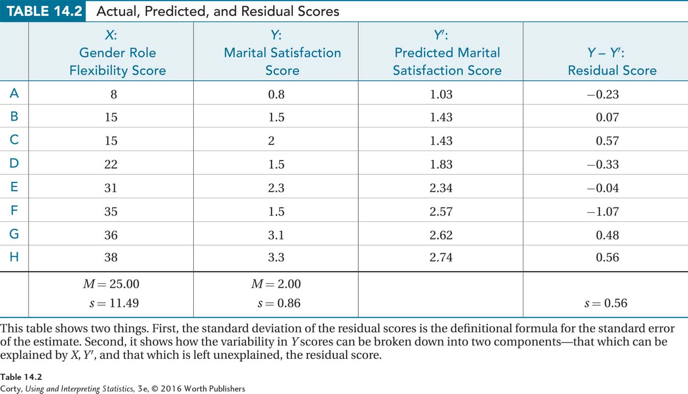
Let’s use Dr. Paik’s marital satisfaction data set, with only eight cases, to calculate the standard error of the estimate. The first two columns in Table 14.2 contain his data set and the third column the predicted Y values for each of the X values. Case A, for example, has a gender role flexibility score of 8 and a marital satisfaction score of 0.8. Using the linear regression equation, its predicted marital satisfaction score is 1.03. The final column is labeled residual scores. It shows the deviation of the predicted score from the actual score, calculated as Y – Y′. The predicted Y score for case A was off by 0.23 points and, because of the direction of the difference, is reported as –0.23. This difference is a measure of how wrong the predicted score is, so it is a measure of error. Case B, for example, where the predicted score was off from the actual score by 0.07 points, had less error in its predicted score than case C, where Y – Y′ was off by 0.57 points.
553
The last column contains deviation scores (error scores), which sum to zero. So, how can the average amount of error be represented? With a standard deviation! And that is what a standard error of the estimate is, the standard deviation of the residual scores. As can be seen at the bottom of the column, for Dr. Paik’s data, the standard deviation of the residual scores, the standard error of the estimate, is 0.56.
The definitional formula requires that we calculate the standard error of the estimate as the standard deviation of the residual scores. Equation 14.4 gives the easier-to-use computational formula, a formula that can be used as long as one knows r and sY .
Equation 14.4 Formula for the Standard Error of the Estimate
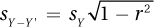
where sY–Y′ = standard error of the estimate
sY = standard deviation of the Y scores
r = the Pearson r value
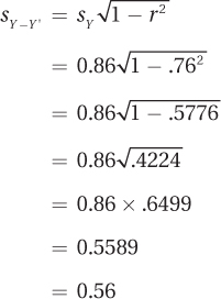
This equation says that the standard error of the estimate may be calculated by (1) squaring the correlation coefficient, (2) subtracting the square from 1, (3) taking the square root of the difference, and (4) multiplying this square root by the standard deviation of the Y scores. Here are the calculations for Dr. Paik’s data. The value about to be calculated, sY–Y′ = 0.56, is exactly the same value that was found as the standard deviation of the difference scores in Table 14.2:
554
What does a standard error of the estimate of 0.56 mean? Loosely, one can think of standard error of the estimate as the average residual score, the average difference between the actual Y scores and the predicted Y scores. Is 0.56 a lot of error? It depends on the possible range of scores. Here the variable being predicted is marital satisfaction, which is measured on a scale ranging from 0 to 4. Being off by 0.56 points, on average, on a 4-point scale means being off, on average, by 14%. That’s not good.
Want a concrete example? Suppose Neil goes to a county fair and stops at an “I’ll Guess Your Weight” booth. The carny guesses Neil’s weight as 150 pounds. But, if he’s off by 14%, Neil could weigh 171 pounds and the carny underestimated his weight. The error could go the other way as well. The carny could have overestimated Neil’s weight. Maybe Neil only weighs 129 pounds, which is off from 150 by 14% in the opposite direction.
This range, from 129 pounds to 171 pounds, gives the general idea of what a prediction interval is. A prediction interval gives a range within which there is some certainty that a case’s real Y score falls. The calculation of the interval is based on the estimated Y score and the standard error of the estimate. The smaller the standard error of the estimate, the narrower the prediction interval and the better the prediction.
Worked Example 14.2
For another example of calculating the standard error of the estimate, a return to the cigarette smoking and lung function study is in order. In that study, 2,500 smokers reported how many years they had been smoking (M = 22, s = 9) and had their lung function measured as a percentage of normal (M = 76, s =13). There was a strong and statistically significant inverse relationship, r = –.68: the longer people smoked, the lower their lung function. After a regression equation was developed, it was used to predict that a person who had been smoking for eight years would have lungs functioning at 89.72% of normal capacity. How much confidence should we have that this estimate is accurate?
555
The way to answer this is by calculating sY–Y′ using Equation 14.4:
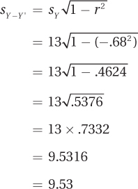
This standard error of the estimate of 9.53 means that the actual Y scores and Y′ scores for the 2,500 people in the sample differed by almost 10 points, on average, on a 100-point scale. That seems like a fair amount of error. This suggests that predictions based on this regression equation aren’t very accurate.
A Common Question
Q So far, both examples have had standard errors of the estimate that are large, suggesting prediction is not very good. What does it take to have a small standard error of the estimate?
A As r grows larger and sY becomes smaller, sY–Y′ gets smaller.
Practice Problems 14.2
Apply Your Knowledge
14.06 Given r = .42 and sY = 5.64, find sY–Y′.
14.07 Dr. Binet developed a regression equation to predict adult IQ from childhood language abilities. IQ can range from 55 to 145. The standard error of the estimate for the regression equation is 14. Is that a large error of the estimate?